The PDURATION function in Google Sheets is used to calculate the number of periods for an investment to reach a specific value, given a specific interest rate.
Table of Contents
This financial function is useful because it helps you find out the amount of time needed to reach a goal amount of money, given an interest rate. It is an easy way to calculate it with the given information.
Let’s look at an example.
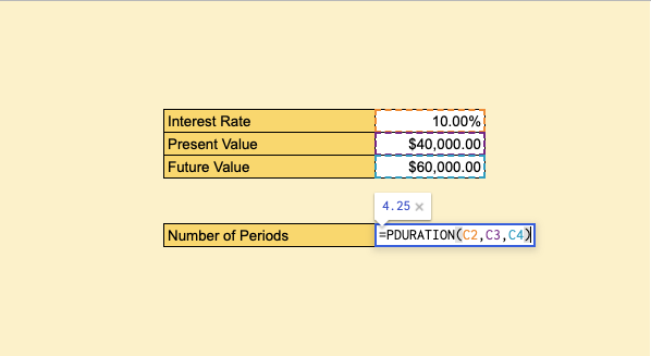
You want to choose to pursue an MBA in the future, and you are calculating your options as you are still working full-time. You decide to make an investment. Given that you can invest $40,000, your goal is $60,000, and the interest rate of the investment is 10%, what is the number of periods required to make the investment reach your desired future value?
How should we go about this problem?
The PDURATION function takes in all these inputs in order to calculate the number of periods.
The Anatomy of the PDURATION Function in Google Sheets
The syntax of the PDURATION function is as follows::
=PDURATION(rate, present_value, future_value)
Let’s have a look at each part of the function to understand what is going on here:
=is the equals sign that starts off any function in Google Sheets.PDURATIONis the name of our function.rateis the rate at which the investment grows with each period.present_valueis the current value of the investment.future_valueis the desired future value for the investment.
Note that all the values must be positive for the function to work. Make sure that all the inputs are greater than 0.
A Real Example of Using the PDURATION Function
Let’s look at the example below to see how to use PDURATION function in Google Sheets.
Calculating the Number of Periods for a Specified Future Value in Google Sheets
This is a simple problem. We want to find the amount of time it will take for the investment to reach the desired future value.

The function takes three arguments, none of which are optional. So in the equation, it will look like:
=PDURATION(C2,C3,C4)
As a result, we get 4.25 years, or 4 years and 3 months.
This simple problem can be practiced to perfection. Use the link below to get a copy of this problem set:
How to Use PDURATION Function in Google Sheets
In this section, we will show you a step-by-step process on how to use the PDURATION function in Google Sheets.
In this problem, we will be calculating the amount of periods it takes to reach the desired future value.
Calculating Amount of Periods in Google Sheets
- To begin, click on a cell to make active, which you would like to display the amount of periods. For this guide, the PDURATION will be in Cell C7.

- Next, type the equal sign ‘=’ to start writing the function. Follow this with “PDURATION” or “pduration” – Google Sheets functions are not case sensitive, so either is fine.

- The auto-suggest box will create a drop-down menu. Select the PDURATION function by clicking it. It is the first to pop up on the list, but take care to choose the correct function.

- After the opening bracket ‘(‘, you will add the rate attribute.

- Next, we enter the present value.

- Next, we enter the desired future value of the investment. You should even see a preview for the end result.

- Hit Enter and you will find the number of periods.

Given a practical problem where you should solve for the correct number of periods, use the PDURATION function to find and study the interest rates and future values for your important financial decision-making.
And there you have it – you can now use the PDURATION function in Google Sheets together with the other numerous Google Sheets formulas to create even more effective formulas.