How to Fix INDEX MATCH Not Returning Correct Value in Excel

This guide will discuss how to fix INDEX MATCH not returning the correct value in Excel. 

The INDEX function and MATCH function in Excel is powerful tools that can be more efficient than the VLOOKUP function. So the combination of the two functions  INDEX MATCH is famous and preferred by many users. 

Essentially, INDEX MATCH works similarly with the VLOOKUP function. So it pulls a value from the selected column based on the given lookup value or criteria. 

And INDEX MATCH has many advantages. One is the ability to choose manually which column to pull from. But, this does not make INDEX MATCH a perfect combination. 

The INDEX MATCH still encounters a few errors and issues when being used. And there could be many possible reasons for the errors. 

Let’s take a sample scenario where the INDEX MATCH is not returning the correct value in Excel. 

Suppose you are making an employee directory containing the employee ID and name. And you were asked to create a separate table for certain employees. So you decided to use INDEX MATCH to pull the names of the employees based on their employee ID. 

But you realized that the returned value was incorrect. What could be the possible reason for this error, and how can you fix it?

Before we answer that question, let’s first dive into the syntax of the INDEX function and MATCH function to understand them better.

The Anatomy of the INDEX Function

The syntax or the way we write the INDEX function is as follows:

=INDEX(array;row_num;[column_num])

Let’s take apart this formula and understand what each term means:

• = this is how we start any function in Excel.
• INDEX() is our INDEX function. This function will return a reference of a cell or value from a particular row and column based on the given range.
• array is a required argument. So this refers to a range of cells or an array constant.
• row_num refers to the selected row in the array or reference from where we will return a value. And this is a required argument. But when omitted, the column_num will be required. 
• column_num refers to the selected column in the array or reference from where the returned value is obtained. Furthermore, this is required when the row_num is omitted.

The Anatomy of the MATCH Function

The syntax or the way we write the MATCH function is as follows:

=MATCH(lookup_value; lookup_array; [match_type])

Let’s dissect this formula and understand what each term means:

• = the equal sign is how we start or activate any function in Excel.
• MATCH() this is our MATCH function. This function will return the relative position of a data or item in an array that matches the given value in a given order. 
• lookup_value refers to the value we use to identify or find the value we want to pull from the array. So this can be a text, number, logical value, or even a reference to any of those. Additionally, this is a required argument. 
• lookup_array is another required argument. And this refers to a range of cells containing possible values we want to pull. So this can be a reference to the array or an array of values.
• [match_type] is an optional argument. So this can either be 1, 0, or -1, which refers to what kind of return value we want. Additionally, 1 will find the largest value that is less than or equal to the given lookup_value. While 0 refers to an exact match to the lookup_value. And -1 will find the smallest value that is greater than or equal to the given lookup_value.

Great! We have learned the syntax of the INDEX MATCH function. Now let’s move on to a real example of how to fix INDEX MATCH not returning the correct value in Excel.

A Real Example of Fixing INDEX MATCH Not Returning Correct Value in Excel

Let’s say we want to pull from the employee directory specific employee names based on their employee ID. Doing this task manually would take too much time. So we will utilize the INDEX function and MATCH function combination to perform this task easily.

Furthermore, the INDEX MATCH combination would be =INDEX(range;(MATCH(lookup_value;lookup_array;[match_type])).

But for some reason, the returned value is incorrect. And there could be several reasons for this error.

Firstly, we did not indicate a match type. Although it is considered an optional argument, INDEX MATCH would most likely give the incorrect value if we do not specify the match type of the value we want. 

So we simply need to input a match type in our formula. In this case, we want an exact match. Then, we will type in 0.

Secondly, there are blank cells in our directory. Basically, blank cells will cause incorrect values to be returned. To fix this, we simply need to delete the blank cells.

Thirdly, our table and range may not correspond. When we use tables and reference the table name, it may be confusing to give the correct one. So we simply need to use the correct table names to obtain the correct returned value.

Next, we may have provided the wrong array. So we may have provided the wrong array, which does not contain our lookup_value. We need to make sure we are typing in the correct lookup array. And this will give us the correct returned value.

Lastly, the reference is not locked. Essentially, this error comes up when we drag down or across the INDEX MATCH formula. Since we are dragging the formula, the references can be disturbed. To ensure this won’t happen, we need to lock the references by inputting the dollar sign $.

You can make your own copy of the spreadsheet above using the link attached below. 

Awesome! Let’s move on and discuss the process of how to fix INDEX MATCH not returning the correct value in Excel.

How to Fix INDEX MATCH Not Returning Correct Value in Excel

In this section, we will discuss the steps on how to fix INDEX MATCH not returning the correct value in Excel.

1. Firstly, one of the reasons is not providing a match type. So we need to provide the match type. In this case, select the formula and simply add a “0” at the end to indicate we want an exact match. So our formula will become “=INDEX(B2:B11;MATCH(D3;A2:A11;0))”.

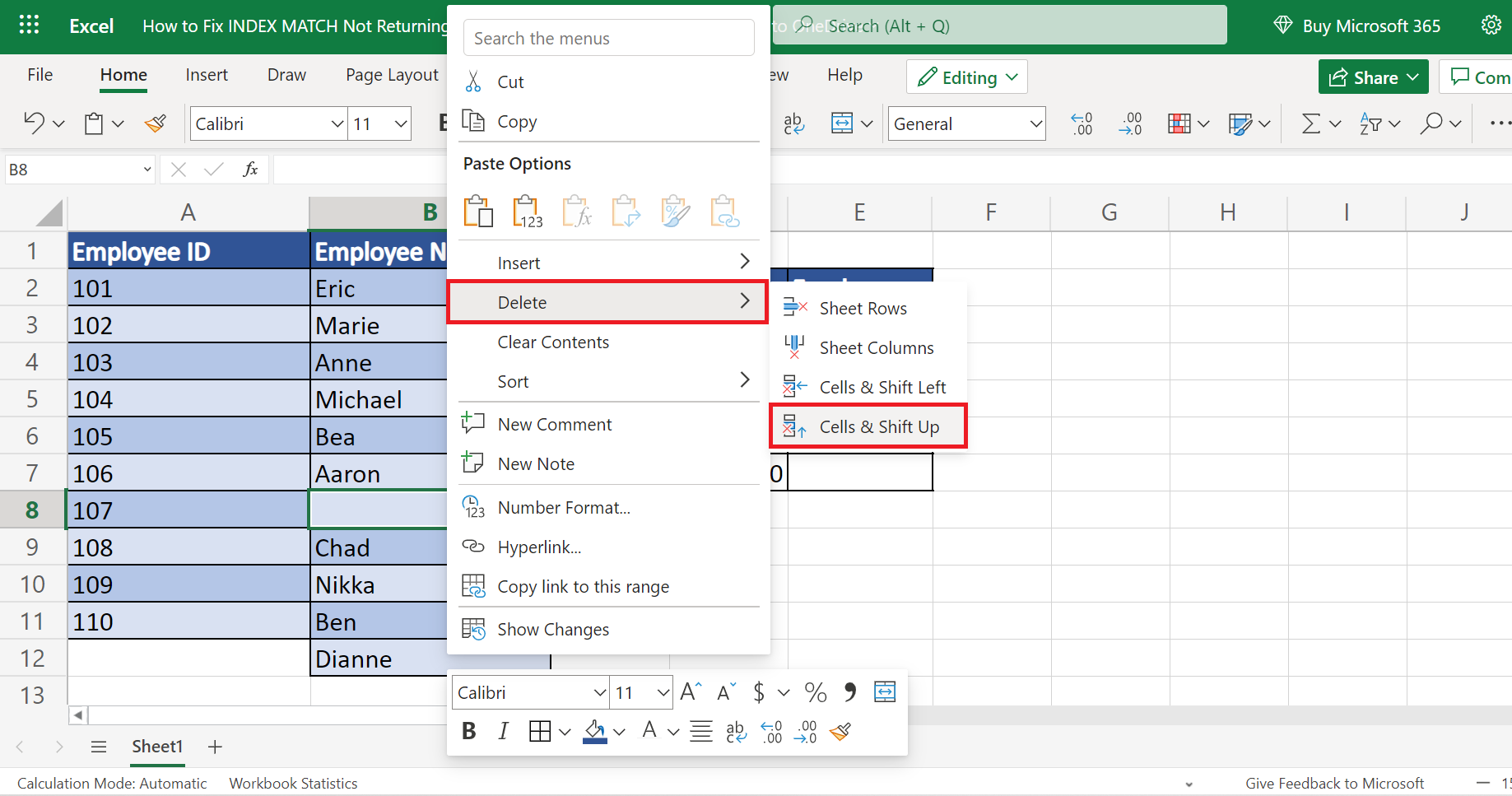
2. Secondly, there may be blank cells left in our table. So select the blank cell and right-click. In the popup menu, click on Delete. Then, another menu will appear. Simply select Cells & Shift Up.

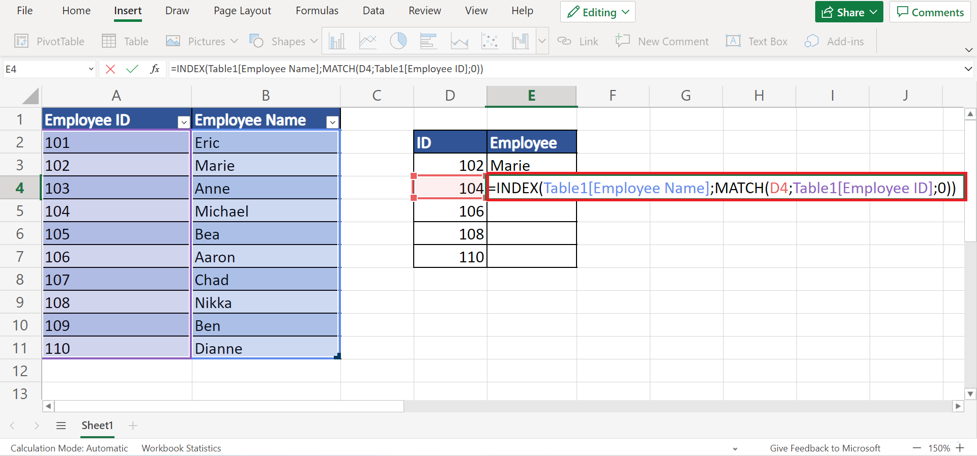
3. Thirdly, input the correct corresponding table and range. In this case, our formula contains the incorrect table name. To fix this, input the correct one. So our formula should be “=INDEX(Table1[Employee Name];MATCH(D4;Table1[Employee ID];0))”.

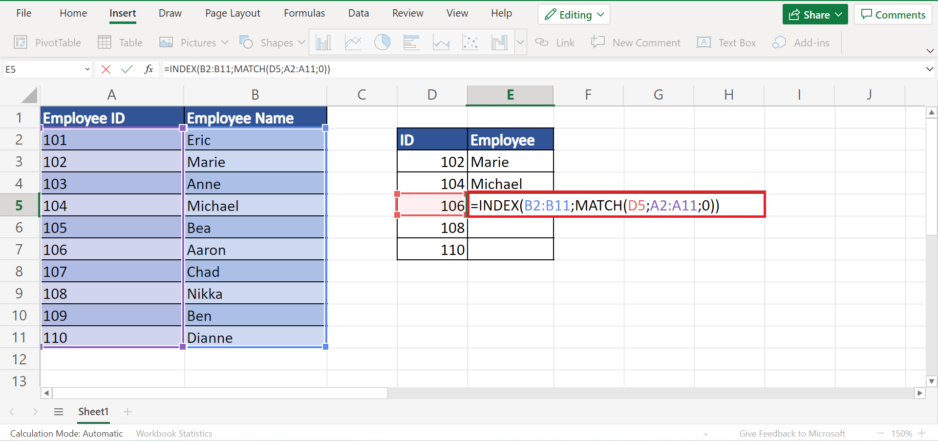
4. Next, we need to provide the correct lookup array. In this case, our lookup value is the employee ID. So our correct lookup array is A2:A12. Then, our correct formula is “=INDEX(B2:B11;MATCH(D5;A2:A11;0))”.

5. Lastly, we need to lock our references. For example, our formula is “. When we drag this formula down or across, we may get incorrect results. So our formula should be “=INDEX($B$3:$B$12;MATCH(D6;$A$3:$A$12;0))”.

6. And tada! We have successfully fixed INDEX MATCH not returning the correct value in Excel in five ways.

That’s pretty much it! Now you can fix INDEX MATCH errors whenever it occurs using the five possible reasons and solutions mentioned above.

Are you interested in learning more about what Excel can do? You can now use the INDEX MATCH functions and the various other Microsoft Excel formulas available to create great worksheets that work for you. Make sure to subscribe to our newsletter to be the first to know about the latest guides and tutorials from us.

Get emails from us about Google Sheets.

Our goal this year is to create lots of rich, bite-sized tutorials for Google Sheets users like you. If you liked this one, you'll love what we are working on! Readers receive ✨ early access ✨ to new content.

Subscribe