This guide will explain how to interpolate missing values in Excel using three easy and simple ways.
Since Excel has several built-in functions and features, we can easily perform challenging tasks. For instance, we can often encounter missing data values whenever we receive a data set. And this may happen for various reasons.
When we encounter missing data values, it is possible to interpolate missing data by estimating the approximate value of those data points using many simple and efficient interpolation techniques.
However, let’s first understand what interpolation is. So interpolation is defined as the process of determining or identifying unknown values that lie in between already known or existing data points. Basically, we will utilize the known data points to fill in the missing data values in our data set.
Furthermore, we will explain three easy and simple methods we can use to interpolate missing values in Excel.
Firstly, we can do the linear trend method. Secondly, we also have the growth trend method. Then, we can utilize the weighted moving average formula. And these methods are applied to different types of data sets.
Once we can determine the type of data set we have and the relationship the values have with each other, we can choose the appropriate method to interpolate missing values in Excel.
Let’s take a sample scenario wherein we must interpolate missing values in Excel.
Suppose you have a data set containing missing interpolated values. And you need to find the missing values to complete your data set. For example, let’s say your data set has a linear pattern. So you can utilize the linear trend method to interpolate the missing values.
Great! Now let’s dive into how to interpolate missing values in Excel using three different methods.
How to Interpolate Missing Values in Excel using the Linear Trend Method
Firstly, we can use the linear trend method. So linear trend refers to whether the data set has variables that follow a constant relationship with each other. Additionally, the rate at which the variables change their values needs to follow a linear pattern.
Moreover, we will be using the linear interpolation formula in this method. So the formula is y = y1 + (x-x1)(y2-y1)/x2-x1. In this formula, (x1, y1) is referring to the first coordinate of the interpolation process. And (x2, y2) refers to the second point of the interpolation process.
Next, x refers to the known value, while y is the unknown value.
If our data set follows a linear pattern, we can use this method to interpolate missing values in Excel. To do this, we can simply follow the steps below.
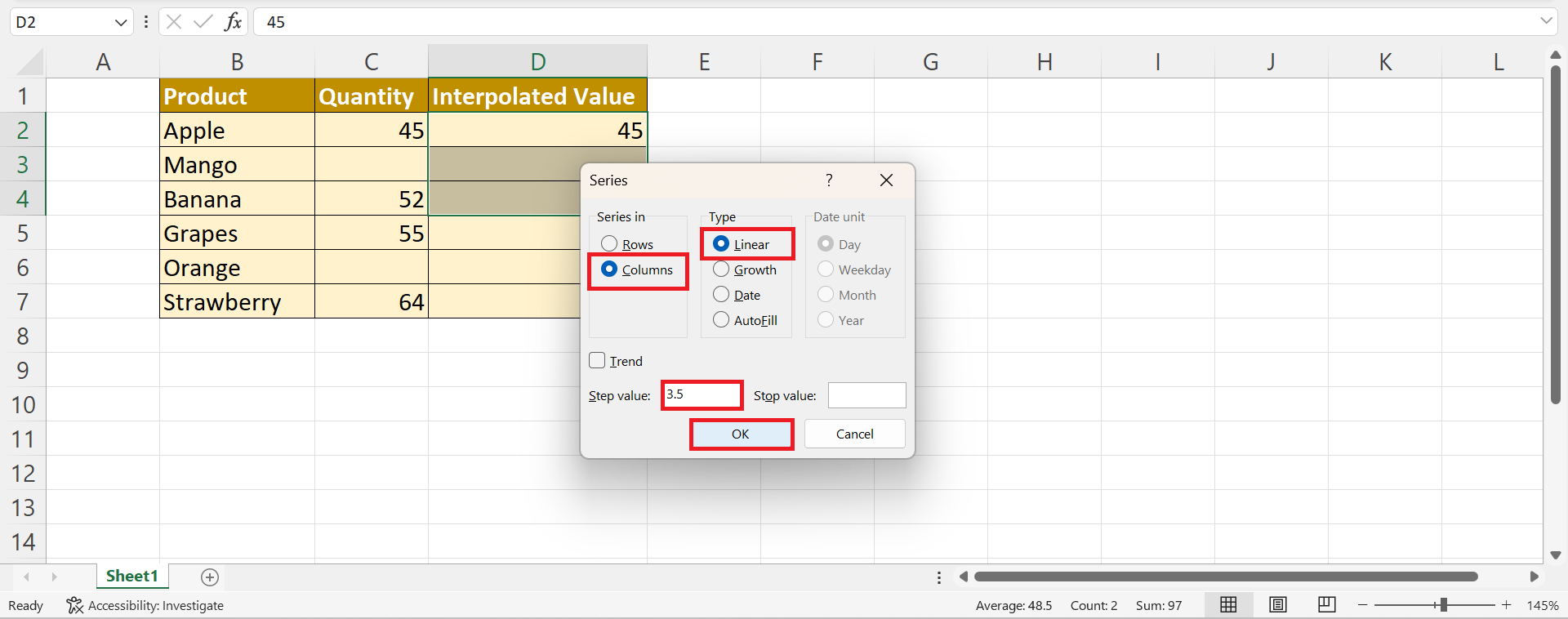
1. Firstly, we need to use the surrounding values to determine the missing values. To do this, we will select the cells and go to the Home tab. Then, we will select the Editing dropdown menu. Next, we will select Fill and click Series.

2. Once the Series window appears, we will select Columns in the Series option. Then, we will select Linear in the Type option. Since we have a different Step value in the data set, we will input “3.5”. Lastly, we will click OK to apply all the options.
3. Afterward, we can simply repeat the process for the other missing cells.
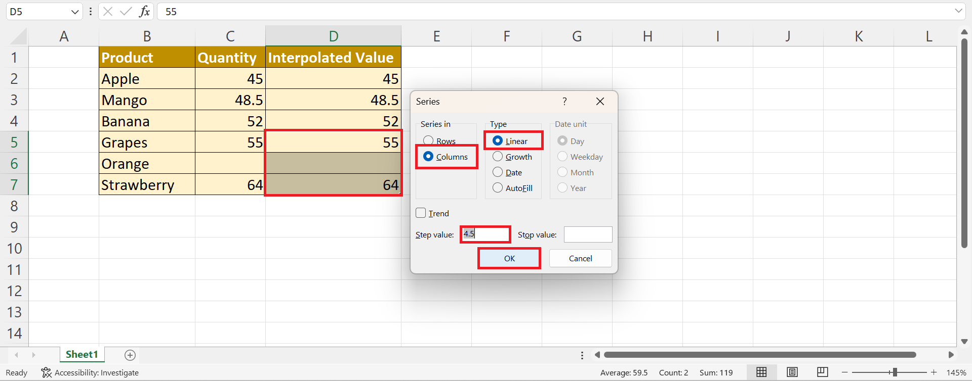
4. And tada! We have successfully used the linear trend method to interpolate missing values in Excel.

How to Interpolate Missing Values in Excel using the Growth Trend Method
Secondly, we will utilize the growth trend method to find the missing values. So this method is used to predict future growth based on past data. Since linear growth suggests a constant extra increase throughout a period of time, this results in a straight path on a chart.
Thus, the annual percentage increase decreases slightly through each passing year.
To apply this method to your data set, we can simply follow the step-by-step process below:
1. Firstly, we will use the known and surrounding values to find the missing values. In this case, the values in cells D3 and D6 are missing. Since the surrounding cells of the missing value are D2 and D4, we will select the range D2:D4. Then, we will head to the Home tab and select Fill in the Editing group.
Next, we will click Series in the dropdown menu.

2. In the Series window, we will select Column in the Series options. Next, we will click Growth in the Type options. Additionally, we will click the checkbox for Trend. Lastly, we will click OK to apply all the changes.

3. Afterward, we can repeat the same process for other missing values.

4. And tada! We have successfully used the growth trend method to interpolate missing values in Excel.

How to Interpolate Missing Values in Excel using the Weighted Moving Average Formula
Thirdly, we can use the weighted moving average formula to determine the missing values. So the weighted moving average formula is a type of metric that is used to give more weight to the latest data point and less weight to the data sets from the past or previous time.
So the formula for the weighted moving average is = A1*W1 + A2*W2 + … + An*Wn) / ΣWt. In this case, A1, A2, and An refer to the data points in the data set. Then, W1, W2, and Wn refer to the weight assigned to each data point. Lastly, ΣWt means the summation of all weights.
And the formula will multiply each number in the data set by a fixed weight and will add the results. So the recent data points have more weight, while the previous data points have less weight.
Additionally, we will use the SUM function with the weighted moving average formula to interpolate the missing values. To use this method, we can follow the steps below.
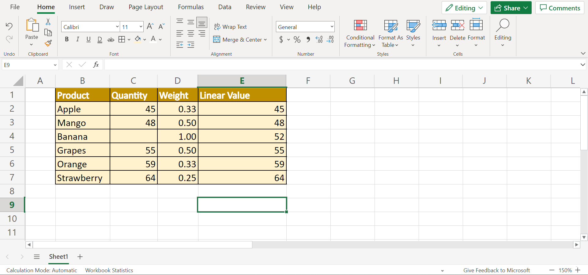
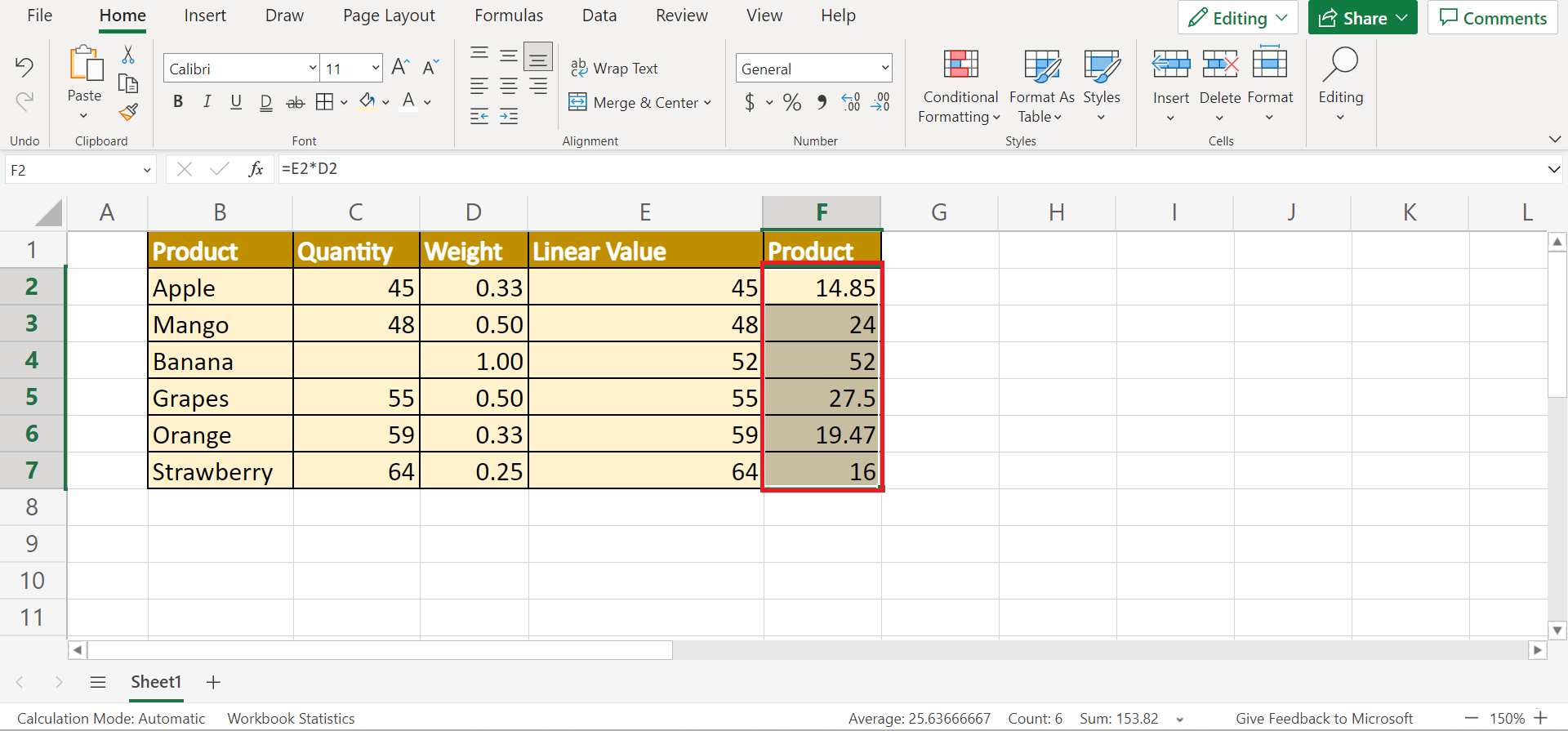
1. Firstly, we will add weight values to each data point. In this case, we will input a weight of “1.00” to our missing value and a weight of “0.50” to the surrounding values. Then, we will input weights of “0.33” and “0.25” to the top and bottom values of the data set.
Next, we will use the interpolated values we have calculated in the previous methods.
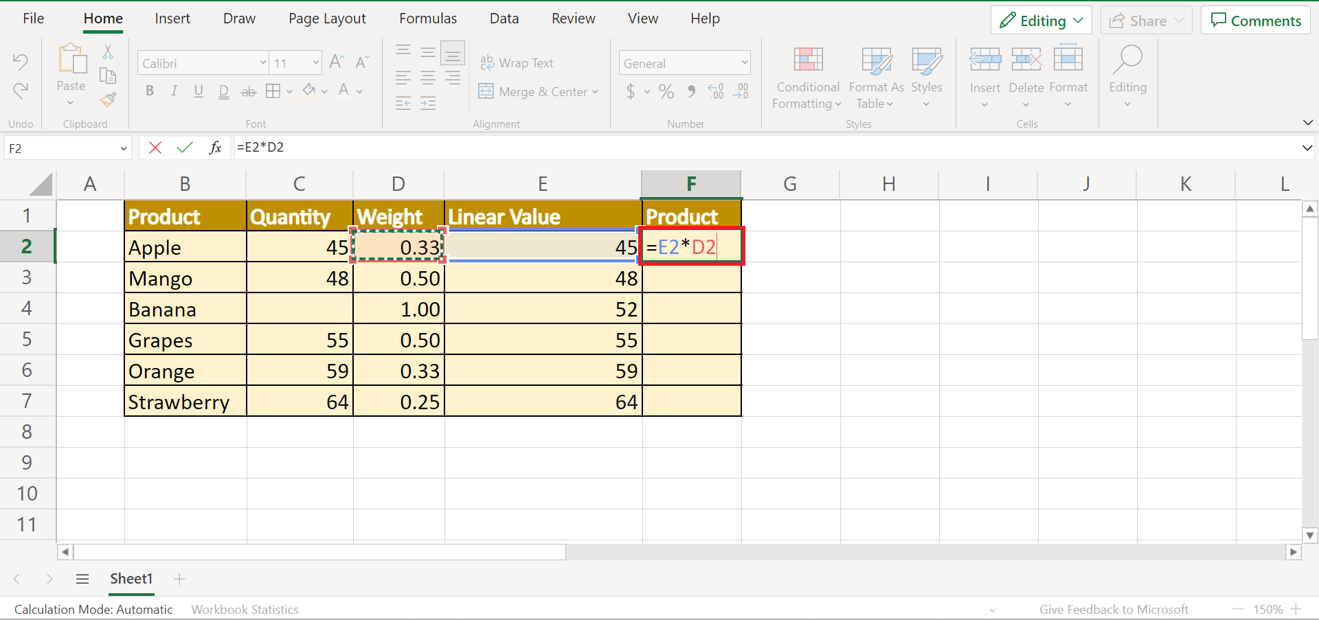
2. Secondly, we will input the formula “=E2*D2” in cell F2. Then, we will press the Enter key to return the value.
3. Thirdly, we will drag down the Fill Handle tool to the other cells in the column.
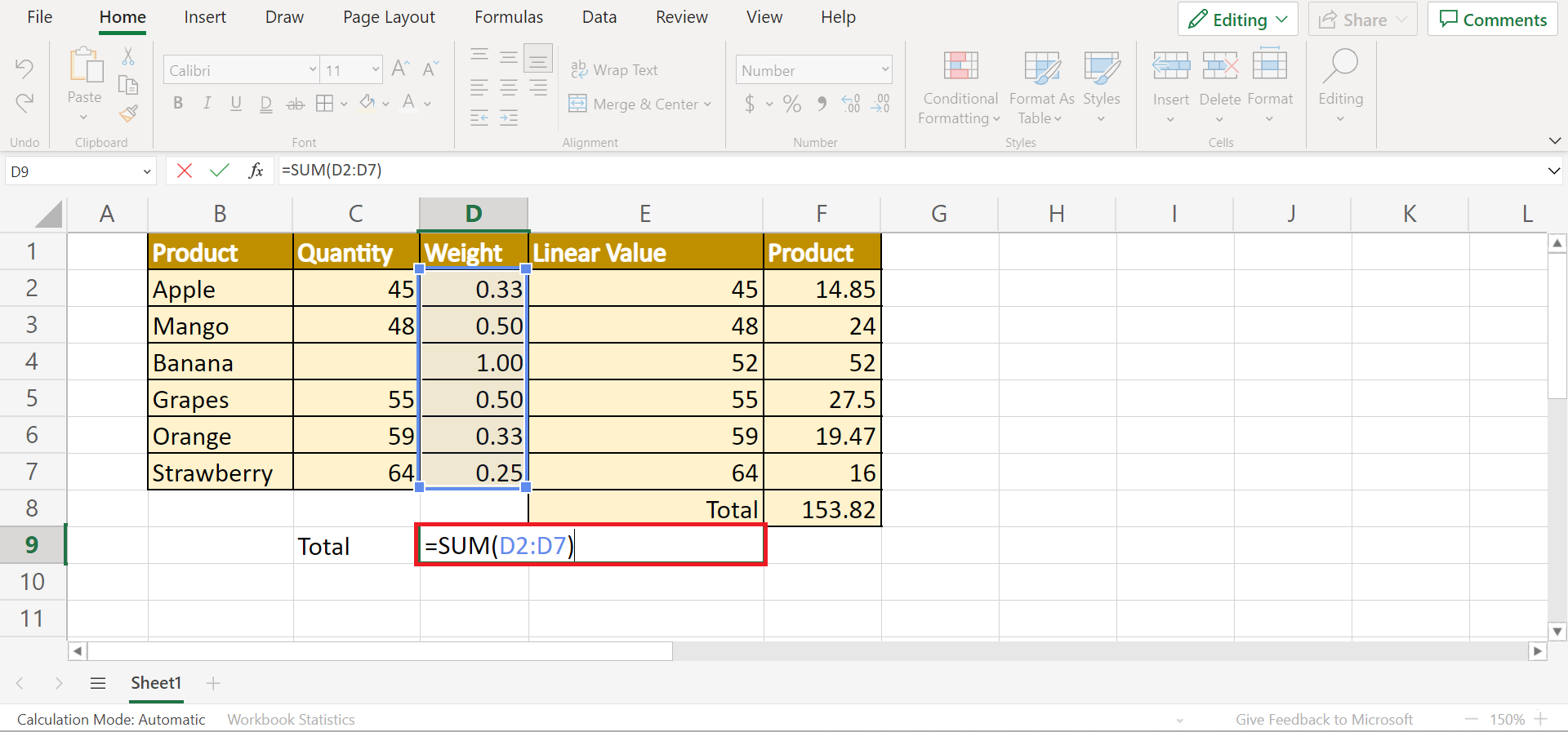
4. Now that we have multiplied the weight and linear values, we can proceed to use the SUM function to get the total. So we will type in the formula “=SUM(F2:F7)”. Lastly, press the Enter key to return the result.

5. Next, we need to get the total weights. To do this, type in the formula “=SUM(D2:D7)”. Lastly, press the Enter key to return the value.
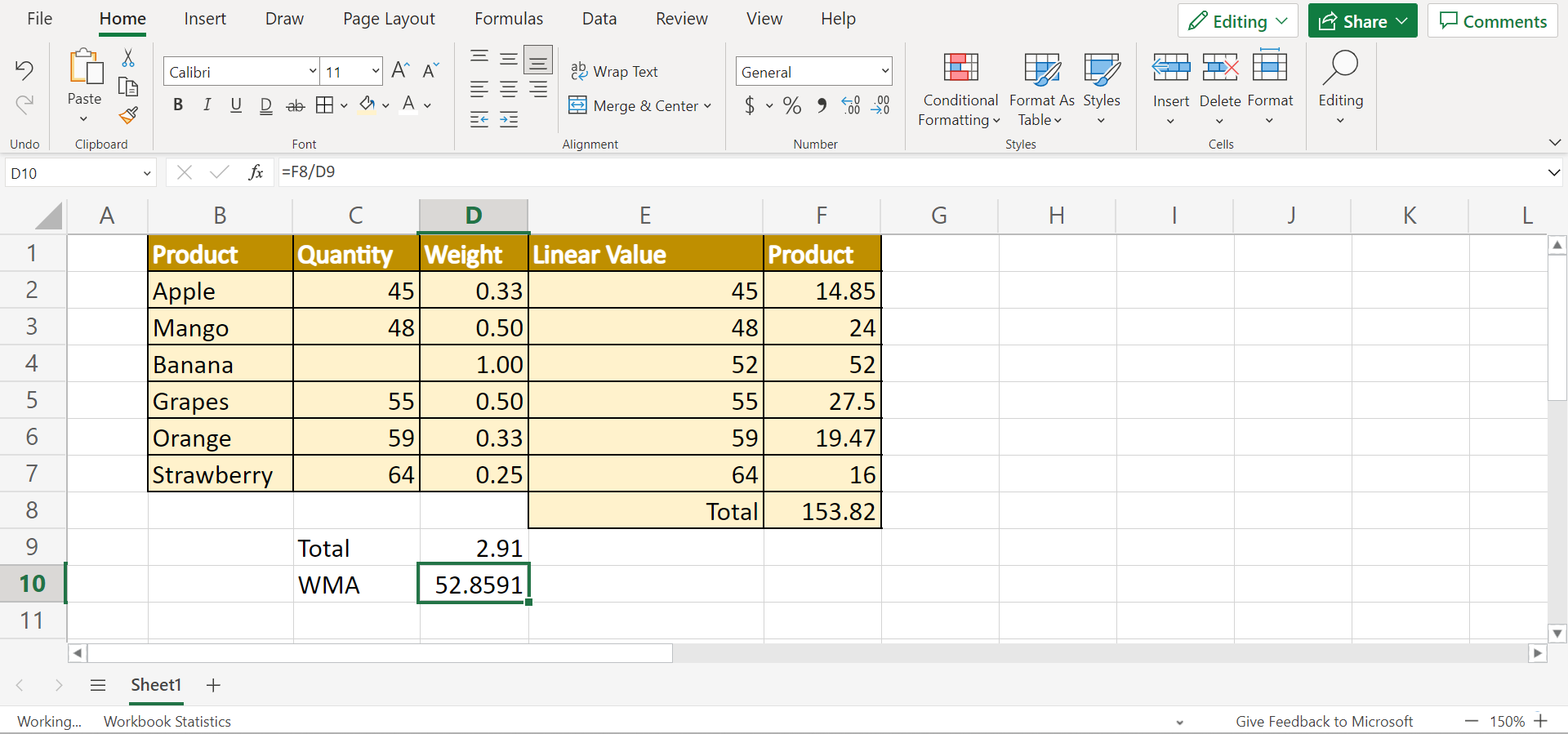
6. Once we have the summation of the weights, we can proceed to get the weighted moving average. So we will input the formula “=F8/D9”. Finally, we will press the Enter key to get the value.

7. And tada! We have found the missing value in the data set.
You can make your own copy of the spreadsheet above using the link attached below.
And that’s pretty much it! We have explained how to interpolate missing values in Excel using three easy and simple methods. Now you can simply choose any of the methods which fit the type of data set you have and fill in the missing values.
Are you interested in learning more about what Excel can do? You can now use the SUM function and the various other Microsoft Excel formulas available to create great worksheets that work for you. Make sure to subscribe to our newsletter to be the first to know about the latest guides and tutorials from us.