This guide will discuss how to sum a range with errors in Excel using three simple and easy methods.
Excel is an excellent tool containing many different functions and tools. And Excel makes the entire process for us easier with these functions. But, sometimes we commit an error in inputting data while performing calculations.
And Excel immediately shows or displays messages to inform or alert us that there is an error in our calculations or data set. But, this also means we cannot get the correct result or even continue performing the function when an error occurs.
In this case, we will focus on performing a sum in a range in Excel. And there are a few methods we can use to still be able to sum a range with errors in Excel.
Let’s take a sample scenario.
Suppose you are performing calculations in Excel. And you are about to sum a range, but you cannot continue because there is an error within the range. Because you have been doing calculations for a long time, you do not want to go back from the top to fix the error.
Worry not! There are a few functions in Excel we can use to sum a range with errors. But before we learn how to do these three simple and easy methods, let’s first discuss the syntax of these functions.
The Anatomy of the AGGREGATE Function
The syntax or the way we write the AGGREGATE function is as follows:
=AGGREGATE(function_num,options,array,[k],...)
Let’s take apart this formula and understand what each term means:
- = the equal sign is how we start any function in Excel.
- AGGREGATE() this is our
AGGREGATEfunction. And this function will return an aggregate in a list. - function_num is a required argument. And this refers to the number 1 to 19 that specifies the summary function for the aggregate.
- options is also a required argument. And this refers to the number 0 to 7 that specifies the values to ignore for the aggregate.
- array is another required argument. And this refers to the array or range containing numerical data on which we will calculate the aggregate.
- k is an optional argument. And this indicates the position in the array, such as k-th largest, k-th smallest, k-th percentile, or k-th quartile.
The Anatomy of the SUMIF Function
The syntax or the way we write the SUMIF function is as follows:
=SUMIF(range,criteria, [sum_range])
Let’s dissect this formula and understand what each term means:
- = the equal sign is how we activate any function in Excel.
- SUMIF() this is our
SUMIFfunction. And this function will add the cells specified by a given condition or criteria. - range is a required argument. And this refers to the range of cells containing the values we want to evaluate
- criteria is also a required argument. And this refers to the criteria or condition in the form of a number, expression, or text which defines the cells added.
- sum_range is an optional argument. So it refers to the actual cells to sum. When we omit this, the function will use the cells in the range.
Awesome! Now that we have dissected some of the functions we will be using, let’s move on and discuss the three simple and easy methods we will use to sum a range with errors in Excel.
How to Sum a Range with Errors in Excel using the AGGREGATE function
The first method we will try is by using the AGGREGATE function. So the AGGREGATE function ignores the N/A errors and will simply proceed to get the sum of the range.
To do this method, follow the steps below:
1. Firstly, we must select a cell to input the results. In this case, let’s input the results into the cell. Then, type in an equal sign to start the AGGREGATE function. So our entire formula would be “=AGGREGATE(9,6,C2:C7)”. Lastly, press the Enter key to return the results.

2. And tada! We successfully sum a range with errors in Excel using the AGGREGATE function.

How to Sum a Range with Errors in Excel using the SUMIF function
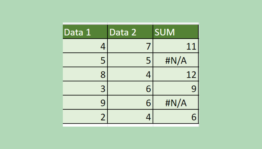
Secondly, we can use the SUMIF function to sum a range with errors in Excel. And this is a relatively simple formula and process. But, this method will only work if the errors present in your data set are N/A errors.
So we simply need to use the not equal operator (<>) with the N/A errors to sum the range. If the data set contains N/A errors, the SUMIF function will return the sum of values not equal to N/A.
To do this method, let’s learn the steps below:
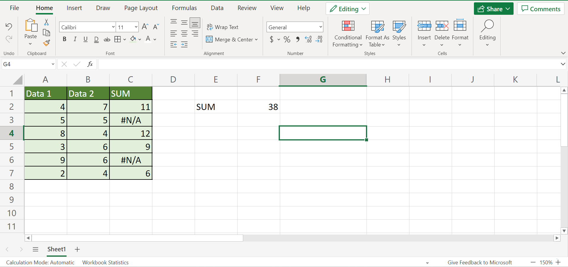
1. Firstly, we must select a cell to input the results. In the same cell, type in an equal sign and the SUMIF function. Then, our entire formula would be “=SUMIF(C2:C7,”<>N/A”)”. Lastly, press the Enter key to return the sum of the range.

2. And tada! We got the sum of a range with errors in Excel using the SUMIF function.
How to Sum a Range with Errors in Excel using the SUM and IFERROR functions
And the last method we will be trying is with the use of the SUM function and the IFERROR function. So this method will create a more literal array formula with the combination of the two functions.
Basically, the IFERROR function traps the errors and converts them to zeros. Then, we can use the SUM function as the errors have been converted to zero.
To do this method, let’s follow the step-by-step process below:
1. Firstly, we must select a cell to input the results. In the same cell, input the formula “=SUM(IFERROR(C2:C7,”0″))”. Lastly, press the Enter key to return the results.

2. And tada! We have sum a range with errors in Excel using the combination of the IFERROR function and the SUM function.
You can make your own copy of the spreadsheet above using the link attached below.
And that’s pretty much it! We have discussed three simple and easy methods to sum a range with errors in Excel. Now you can apply any of these methods whenever you encounter the same issue.
Are you interested in learning more about what Excel can do? You can now use the SUMIF function, AGGREGATE function, and the various other Microsoft Excel formulas available to create great worksheets that work for you. Make sure to subscribe to our newsletter to be the first to know about the latest guides and tutorials from us.