This guide will explain how to use the PMT function in Excel.
The rules for using the PMT function in Excel are the following:
- When the given rate value is less than or equal to -1, the
PMTfunction returns a #NUM! error. - When the nper value is equal to 0, the
PMTfunction returns a #NUM! error. - When any of the arguments given is non-numeric, the
PMTfunction returns a #VALUE! error. - We need to convert the number of periods to months or annual interest rates to months or quarters.
Excel is an extremely useful tool containing several functions which can be used for several calculations and tasks. And one of these functions is the PMT function in Excel.
So the PMT function is used to calculate the payment for a loan based on constant payments and a constant interest rate. And PMT stands for payment. Furthermore, this function is mostly used for financial purposes to figure out payments for a loan.
Let’s take a sample scenario.
Suppose you took out a car loan. And you want to calculate how much you have to pay for your loan on a monthly basis. So this is where you can utilize the PMT function to simply and quickly get the monthly payment amount.
Great! Before we discuss a real example of using the PMT function in Excel, let’s first understand the syntax of the PMT function.
The Anatomy of the PMT Function
The syntax or the way we write the PMT function is as follows:
=PMT(rate, nper, pv, [fv], [type])
Let’s take apart this formula and understand what each term means:
- = the equal sign is how we start any function in Excel.
- PMT() this is our
PMTfunction. And this function is often used for financial aspects such as interest rates and calculating loan payments. - rate is a required argument. And this refers to the interest rate per period for the loan.
- nper is also a required argument. And this refers to the total number of payments for the loan.
- pv is another required argument. And it refers to the present value, meaning the total amount the future payments are worth now.
- fv is an optional argument. And it refers to the future value you want to attain after the last payment is made. Additionally, this will be 0 if omitted.
- type is another optional argument. And it refers to a logical value or the payment made at the start of the period.
Awesome! Now let’s move on and discuss a real example of using the PMT function in Excel.
A Real Example of Using the PMT Function in Excel
Let’s say we want to invest in the business. And assuming that we will receive an amount of $100,000 after three years. In this case, our rate of interest is 4% per year, and the payment will be made at the start of each month.
So this is what the details of our PMT function would look like:

Afterward, we can simply utilize the PMT function and input the necessary arguments based on the given values to obtain the amount for our monthly investments.
Lastly, we will obtain the final result, which is $2,952.42. So this will be the monthly investment we need to pay at the start of each month.

You can make your own copy of the spreadsheet above using the link attached below.
Great! Now let’s dive into the step-by-step process of how to use the PMT function in Excel.
How to Use the PMT Function in Excel
In this section, we will explain the step-by-step process of how to use the PMT function in Excel. Furthermore, each step will contain a detailed explanation and pictures to guide you along the process.
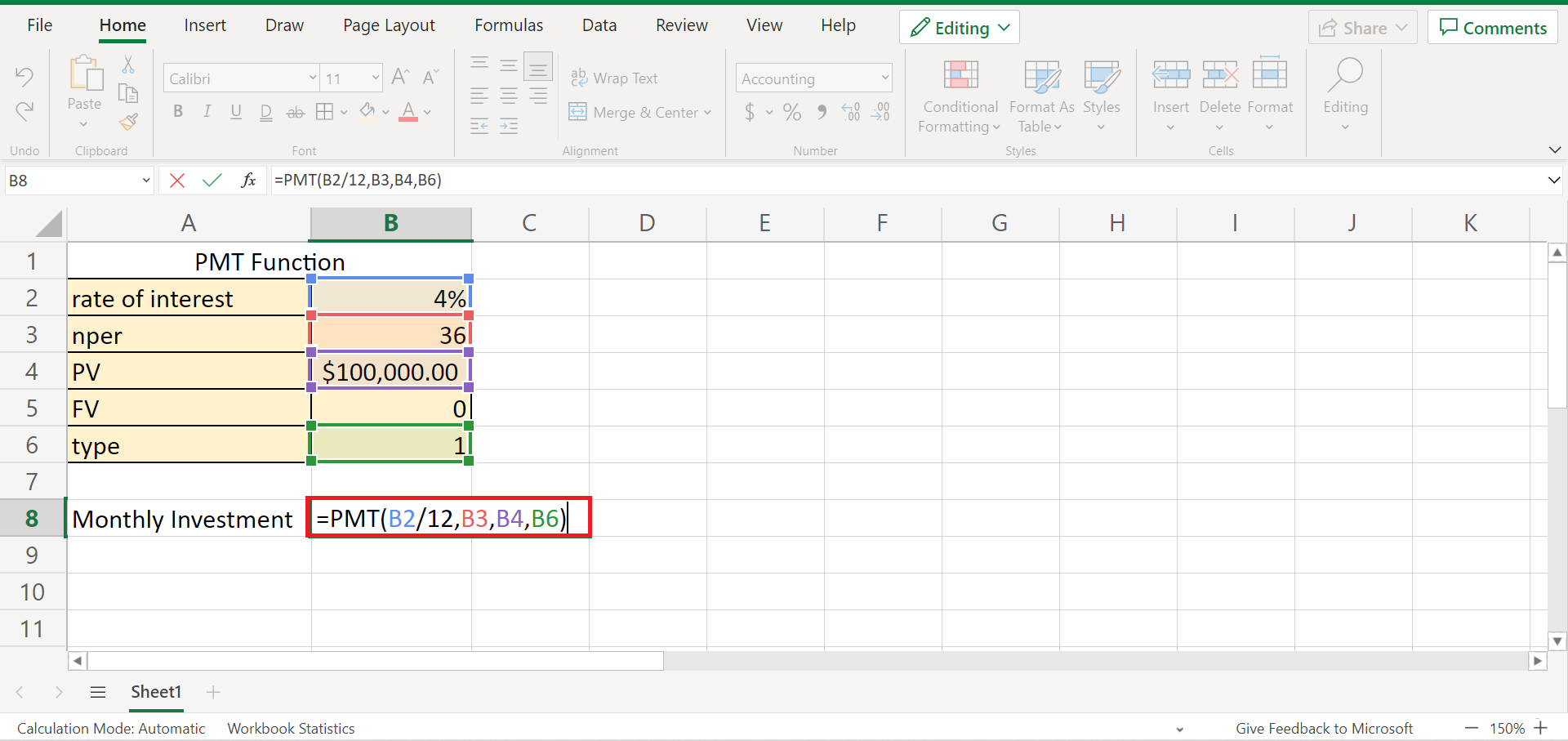
1. Firstly, we must create a table of values for the necessary component to calculate the PMT function. Next, we will input the rate of interest, which is 4%. Then, our nper is 36 because we will only receive the money after 3 years. Next, we will input the present value, which is $100,000.
2. Secondly, we can now perform the PMT function in Excel. First, type an equal sign to start the function and type in the PMT function. Next, select the cell containing the rate of interest, nper, and PV. So our entire formula would be “=PMT(B2/12,B3,B4,B6)”. Lastly, press the Enter key to return the result.
3. And tada! We have successfully used the PMT function to calculate the monthly investment amount.
And that’s pretty much it! So we have discussed the rules of using the function, the syntax of the PMT function, and the steps on how to use the function in Excel. And now, you can apply this learning whenever you need to.
Are you interested in learning more about what Excel can do? You can now use the PMT function and the various other Microsoft Excel formulas available to create great worksheets that work for you. Make sure to subscribe to our newsletter to be the first to know about the latest guides and tutorials from us.