How To Use ISNA Function in Google Sheets

The ISNA function in Google Sheets is useful when you need to check whether the value of a cell is the ‘#N/A’ error.

The #N/A or “value not available” error indicates that there is missing information that stops the function from calculating.

The rules for using the ISNA function in Google Sheets are as follows:

• The cell reference containing the value to check is our sole argument for the ISNA function.
• The function then outputs TRUE when the value of the argument is the #N/A error and FALSE otherwise.
• The #N/A error can be caused by a function requiring three arguments that were only provided with two arguments, or by a function like VLOOKUP that is unable to find a given search term.

Let’s look at a quick example! 

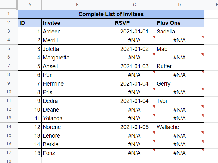
For example, let’s say we’re planning a formal event. We have a list of guests who have been invited and another list with confirmed RSVPs. The second list also contains an invitee’s plus-one. As the planner, you would like to see which of the invitees have confirmed RSVPs and plus-ones. You’ve decided to use the VLOOKUP function to set up a table, but it ends up looking like this.

Using the ISNA function, we can write a formula that expects these kinds of errors. For instance, if a guest in List A cannot be found in List B, then output ‘Pending’ or a placeholder text like ‘-’.

This use case is just one way to use the ISNA function in Google Sheets. The function can help make your datasets look cleaner and can allow you to work with data even if functions like VLOOKUP fail.

Now that we know when to use the ISNA function, let’s dive into how to use it and work on an actual sample spreadsheet.

The Anatomy of the ISNA Function

So the syntax (the way we write) of the ISNA function is as follows:

=ISNA(value)

Let’s dissect this thing and understand what each of these terms means:

• = the equal sign is how we start any function in Google Sheets.
• ISNA() is our ISNA function. It returns whether the given argument is the #N/A error.
• value refers to the value to be compared with the error value #N/A
• This function is often used together with the IF function in conditional statements.

A Real Example of Using ISNA Function

Let’s look at an example of the ISNA function in Google Sheets.

The example below shows the two lists mentioned in the previous section. The leftmost table shows a list of invitees as well as their RSVP status and the name of their plus-one. Adding a new confirmed entry to the list on the right will automatically update the list on the left.

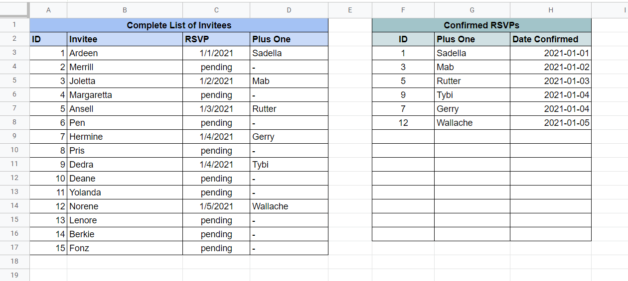
To get the values in Column C, we just need to use the following formula:

=IF(ISNA(VLOOKUP(A3,$F:$H,3,FALSE)),"pending",VLOOKUP(A3,$F:$H,3,FALSE))

You can make a copy of the spreadsheet above using the link I have attached below. 

If you’re ready to test the ISNA function in Google Sheets, let’s start writing it step-by-step!

How to Use ISNA Function in Google Sheets

In this guide, we’ll be using a simplified version of the sample sheet above. In this case, we only want to know if a given invitee has a confirmed RSVP or not. Thus, the value of the column must be either TRUE or FALSE.

1. First, we must find the cell which may produce #N/A errors. In the example below, Column C uses VLOOKUP, which may return such an error.
   
   
   
2. Next, we can rewrite the formula to handle the #N/A error by wrapping the ISNA error around the current formula. If a guest does not appear in the Confirmed RSVPs list, it will return TRUE.
   Since we’re looking for a value of FALSE, in that case, we must invert the result using the NOT function.
   
    
3. Afterward, just hit the Enter key on your keyboard to let the function evaluate. 
4. Finally, we can drag down the formula to fill out the rest of the column.
   
    
5. If you want to return the value of the VLOOKUP as well, we can use a more complex formula, as seen below.
   

Frequently Asked Questions (FAQ)

1. Will this formula detect other types of errors?
   The ISNA function only works with #N/A errors. Any other error will cause the function to return FALSE. If you need to check for errors other than #N/A, you may use the ISERR function instead.  
2. Is there a way to return the #N/A error without using other formulas?
   For cases when you would like to test your ISNA formula, you can return the “value not available” error by using the NA function. 

This step-by-step guide shows how easy it is to detect #N/A errors in your worksheet. The ISNA function is the most reliable way to prevent functions with missing arguments from returning unusable data.

You can now use the ISNA function in Google Sheets along with the various other Google Sheets formulas available to create powerful worksheets that work for you. 

Stay notified of new Google Sheets guides like this by subscribing to our newsletter!

Get emails from us about Google Sheets.

Our goal this year is to create lots of rich, bite-sized tutorials for Google Sheets users like you. If you liked this one, you'd love what we are working on! Readers receive ✨ early access ✨ to new content.

Subscribe