The ISDATE function in Google Sheets is useful if you want to know whether the value in a cell is a date or not.
Meaning, the ISDATE function returns TRUE if the value passed to it is a date value. Otherwise, it would return FALSE.
Table of Contents
The rules for using the ISDATE function in Google Sheets are as follows:
- The date must be enclosed with quotation marks if passed as a direct argument.
- If cell reference is used, quotation marks are not necessary.
Let’s take an example.
Ciara needs to check if the submitted birthday values in the form responses are in date format. See the form responses below:

Ciara needs to identify if the birthday information provided is correct based on its format. While she can do it manually, it would still take a lot of time to validate each one of them.
She applied the ISDATE function to each birthday value. This way, she would be able to identify who provided incorrect birthday information so she could get back to them.
See the result of her validation:

Clever, right?
Watch out for a more advanced tutorial and examples on how you can use the ISDATE function in the coming weeks. Be sure to subscribe to be notified.
Perfect! Let’s begin getting to know more about our ISDATE function in Google Sheets.
The Anatomy of the ISDATE Function
So the syntax (the way we write) of the ISDATE function is as follows:
=ISDATE(value)
Let’s dissect this thing and understand what each of these terms means:
- = the equal sign is just how we start any function in Google Sheets. It is how Google Sheets understand that we are asking it to either do computation or use a function.
- ISDATE() is our ISDATE function. It returns whether a value is a date or not.
- value is the value to be verified as a date.
A Real Example of Using ISDATE Function
Let’s take a look at Ciara’s form responses below to see how the ISDATE function is used in Google Sheets.

Like the PROPER, LOWER, and UPPER functions, the ISDATE function is pretty much straightforward. You want to know if a given value is a date? Go ahead and pass it to the ISDATE function and see the magic happens.
In the examples above, the date values to be checked are the birthdate provided by the form submitter. These birthdates are in column C.
Ciara added a new column to evaluate whether the provided birthday values are correct date values or not. In that column, she used the ISDATE function and passed the cell reference as the argument.
For the first entry, she passed cell C2 in the ISDATE function.

Notice that the returned value of the function is TRUE in column D. This means that the ISDATE function considers the value in cell C2 as a valid date, which you can easily notice that it is indeed a valid date value.
Let’s now check the second entry in the form responses.
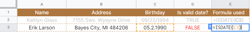
The ISDATE function doesn’t consider the value in cell C3 as a valid date. Hence, it returned a FALSE value in column D.
You can verify that the value in C3 isn’t recognized as a valid date format since it uses a period as the delimiter for the day, month and year.
You may make a copy of the spreadsheet using the link I have attached below.
How to Use ISDATE Function in Google Sheets
- Click on any cell to make it the active cell. For this guide, I will be selecting D2, where I want to show the result.

- Next, type the equal sign ‘=‘ to begin the function and then follow it with the name of the function, which is our ‘isdate‘ (or ‘ISDATE‘, not case sensitive like our other functions).

- Type open parenthesis ‘(‘ or simply hit Tab key to let you use that function.
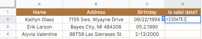
- Now the exciting part! Let’s give our function its only argument, the value. You may pass constant data by typing the exact value after the parenthesis. Just don’t forget to enclose it with quotation marks (“”). In this case, type in ‘09/22/1994’.
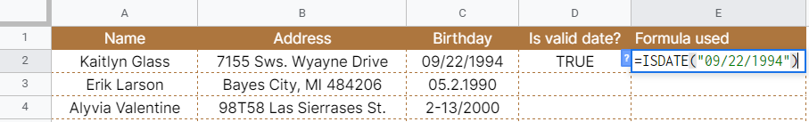
- Finally, hit your Enter or Tab key. Cell D2 will now show you the return value of the ISDATE function.
- Notice that in this example, we provided the exact date value, constant, as the argument of our ISDATE function. Alternatively, this constant can be a variable or simply a cell address containing your value.
- Edit the formula in cell D2 by changing the date value into the cell address. In this case, type in ‘C2’.
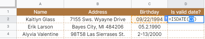
- Hit your Enter or Tab key again. Cell C2 will now show you the same result.
- Copy the formula down to the remaining cells. Rows in column D will now show you whether the date provided in each row in column C is a valid date or not.

That’s pretty much it. You can now use the ISDATE function in Google Sheets together with the other numerous Google Sheets formulas to create even more powerful formulas that can make your life much easier.