The SUMIFS function in Google Sheets is useful if you want to get the sum of cells that meet the two or more provided conditions in a given range.
Meaning, the SUMIFS function adds up cells that meet the given multiple criteria.
Table of Contents
The rules for using the SUMIFS function in Google Sheets are as follows:
- The SUMIFS function supports multiple conditions. On the other hand, the SUMIF function, which we have discussed in our previous article, supports single conditions only.
- The criteria can be based on dates, texts, and numbers.
- The SUMIFS function supports logical operators such as (>,<,<>,=) and wildcards (*,?). For more information on how wildcards are used for the SUMIFS function, please refer to our previous article.
- Each additional range must have the same number of rows and columns as sum_range, but ranges do not need to be adjacent. If you supply ranges that don’t match, you’ll get a #VALUE error.
- The SUMIF and SUMIFS functions require a range, and you can’t use an array.
- Text string in criteria should be enclosed with quotation marks, whereas cell reference shouldn’t.
- Up to 127 range/criteria pairs are allowed to be used in the SUMIFS function.
Let’s take an example.
Gerald has been instructed by his supervisor to prepare reports for the upcoming business review for May.
He has the data below and needs to generate a summary for him to put in the presentation.
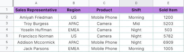
His boss wanted to see the numbers based on the following criteria:

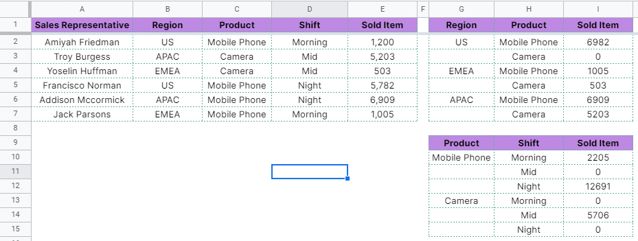
With the help of the SUMIFS function, Gerald was able to yield numbers based on the criteria of his boss.
See his final table below:
Pretty smart, right?
Watch out for a more advanced tutorial and examples on how you can use the SUMIFS function in the coming weeks. Be sure to subscribe to be notified.
Perfect! Let’s begin getting to know more about our SUMIFS function in Google Sheets.
The Anatomy of the SUMIFS Function
So the syntax (the way we write) of the SUMIFS function is as follows:
=SUMIFS(sum_range,range1,criteria1,[range2],[criteria2],...)
Let’s dissect this thing and understand what each of these terms means:
- = the equal sign is just how we start any function in Google Sheets. It is how Google Sheets understand that we are asking it to either do computation or use a function.
- SUMIFS() is our SUMIFS function. It gets the sum of cells that meet the two or more provided conditions.
- sum_range is the range of cells to be summed.
- range1 is the first range to be evaluated.
- criteria1 is the criteria to use in range1.
- [range2] is an optional argument. This is the second range to be evaluated.
- [criteria2] is an optional argument. This is the criteria to use in [range2].
A Real Example of Using SUMIFS Function
Let’s take a look at the reports that Gerald prepared below to see how the SUMIFS function is used in Google Sheets.

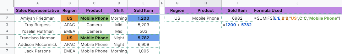
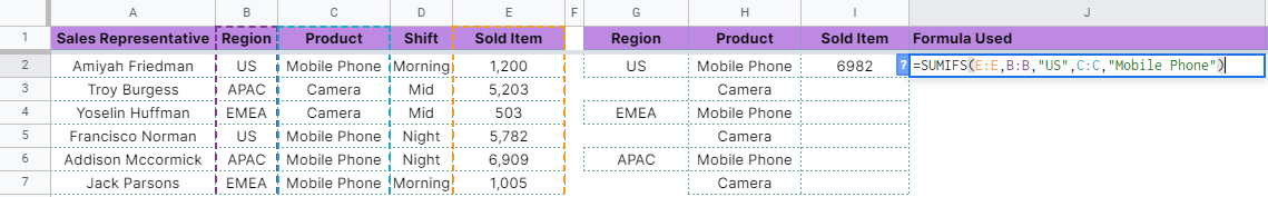
In the first and second criteria that his boss required of him to do, Gerald pulled the total sold mobile phones and cameras per region. He used cell references to the SUMIFS function.
=SUMIFS(E:E,B:B,”US“,C:C,”Mobile Phone“)
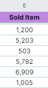
The first argument is column E, which is the column to be summed up. Column E holds the number of sold items per row.
The second argument is column B, which holds the region values. It has three possible values (US, EMEA, and APAC). This is the column where the next argument will be tested against.

The third argument is the text value “US”. Note that the second and third arguments are the first criteria.
=SUMIFS(E:E,B:B,”US“,C:C,”Mobile Phone”)
The criteria are supplied in pairs (range/criteria) and only the first pair is required.
Now, let’s proceed to the next arguments, which are the second criteria in the example above.
=SUMIFS(E:E,B:B,”US“,C:C,”Mobile Phone“)
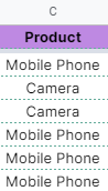
The fourth argument is column C, which contains the text values ‘Mobile Phones’ and ‘Camera’.
Lastly, the fifth argument is the text value ‘Mobile Phone’.
This means that the SUMIFS function will perform addition to cells in column E that correspond to the cells in column B which have the instances of the text string ‘US’ and cells in column C which have the instances of the text string ‘Mobile Phones’
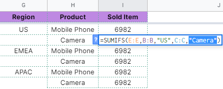
Now, to extract the number of sold cameras in the US region, he changed the text in the fifth argument from ‘Mobile Phone’ to ‘Camera’.
=SUMIFS(E:E,B:B,”US”,C:C,”Camera“)
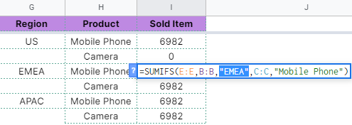
However, the function returns a 0 result.
![]()
Why is this so?
Well, that’s because out of the 2 criteria provided, only the first one was met. Note that for the SUMIFS function to perform the addition, all criteria must be met.
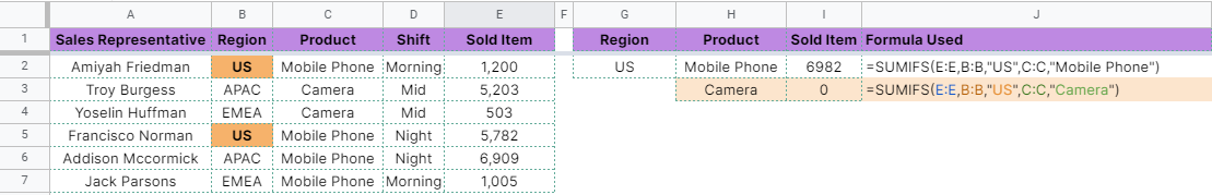
While there are ‘US’ text values in column B, there were no ‘Camera’ values found in column C with the ‘US’ value in column B. Hence, the function returned a 0 value. This means that in the US, no camera phone was sold for May.
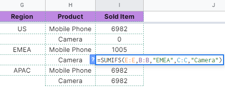
The same logic applies to the SUMIFS function used to pull the numbers for the remaining regions for each product.

Now, let’s take a look at the second report Gerald extracted from his table.
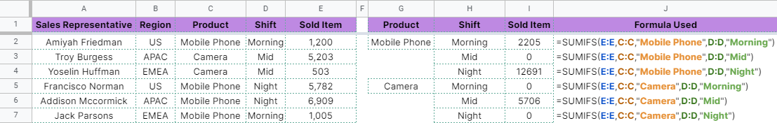
He pulled the total item sold for each product per shift.
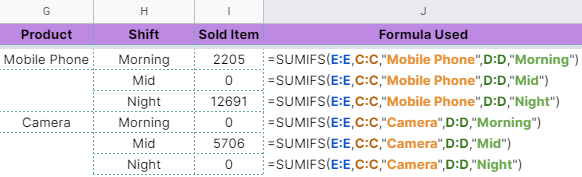
For the mobile phone product, the first argument is column E, which is the column to be summed up. The first pair of criteria is column C and the text value ‘Mobile Phone’ and the second pair of criteria is column D and the text value ‘Morning’.
This means that the function will perform addition to cells in column E that correspond to the cells in column C which have values ‘Mobile Phone’ and to the cells in column D which have the values ‘Morning’.

The same logic applies to the SUMIFS function used to pull the total mobile phones sold for mid and night shifts. See below:

Gerald only changed the values in the fifth argument from ‘Morning’ to ‘Mid’ and ‘Night’.
He never had a hard time getting the number of sold cameras for each shift since he only had to change the formula used above. He simply changed the text in the third argument from ‘Mobile Phones’ to ‘Camera’.

You may make a copy of the spreadsheet using the link I have attached below.
How to Use SUMIFS Function in Google Sheets
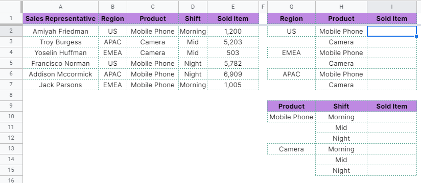
- Click on any cell to make it the active cell. For this guide, I will be selecting I2, where I want to show the result.
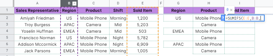
- Next, type the equal sign ‘=‘ to begin the function and then follow it with the name of the function, which is our ‘sumifs‘ (or ‘SUMIFS‘, not case sensitive like our other functions).

- Type open parenthesis ‘(‘ or simply hit Tab key to let you use that function.

- Now the exciting part! Let’s give our function its first argument, the sum_range. Click the range or column that you want to use. In this case, click on column E or type in ‘E:E’.

- To let the Google sheet know that we’re done typing our first argument, we should now type in the delimiter or the character that separates each argument on a function. In this case, type comma ‘,’.

- Type in our second argument, which is the range1. Click on column B or type in ‘B:B’ and follow it with a comma (,).
- Now, pass the third argument, which is the criteria1. Type in the text string ‘US’. Just be sure to enclose it with quotation marks (“”). Alternatively, you may use a cell address that contains the text ‘US’. You may type in ‘G2’ instead of the text string ‘US’. Take note that you don’t have to enclose the cell address to quotation marks. For my example, I’ll use the text ‘US‘ and follow it with a comma (,).

- Provide the fourth argument, which is the [range2]. Click on column C or type in ‘C:C’ and follow it with a comma (,).

- Pass the last argument, which is the [criteria2]. Type in the text string ‘Mobile Phone’. Just be sure to enclose it with quotation marks (“”). Alternatively, you may type in ‘H2’ instead of the text string ‘Mobile Phone’. For my example, I’ll use the text ‘Mobile Phone’.

- Finally, hit your Enter or Tab key. Cell I2 will now show you the return value of the SUMIFS function, or the total mobile phones sold in the US region.
- Copy the formula down to cell I7.

- Update the arguments in each row based on the conditions being asked.
- For the formula in cell I3, change the value in the fifth argument from ‘Mobile Phone’ to ‘Camera’.
- For the formula in cell I4, change the value in the third argument from ‘US’ to ‘EMEA’.
- For the formula in cell I5, change the value in the third argument from ‘US’ to ‘EMEA’ and the value in the fifth argument from ‘Mobile Phone’ to ‘Camera’.
- For the formula in cell I6, change the value in the third argument from ‘US’ to ‘APAC’.

- Lastly, for the formula in cell I7, change the value in the third argument from ‘US’ to ‘APAC’ and the value in the fifth argument from ‘Mobile Phone’ to ‘Camera’.

- Hit your Enter or Tab key. Cells I2-I7 will now show you the return values of the SUMIFS functions with different criteria based on columns G and H.

That’s pretty much it. You can now use the SUMIFS function in Google Sheets together with the other numerous Google Sheets formulas to create even more powerful formulas that can make your life much easier.