When working with Google Sheets, it might be helpful to link data from a different tab in your spreadsheet.
Your projects may grow in size and scope, leading to multiple sheets or even multiple files. This article will explain to you how simple it is to connect data outside of your current sheet.
Let’s look at a scenario where we might need to connect data found in different sheets. In this example, we’re a small business that sells antiques, and paintings online. We have data from the past two years, and we want to know how much growth we have had since last year.
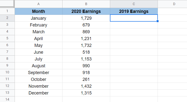
In the sheet below, we have two sheets. The first sheet has a table containing our monthly earnings for 2020.

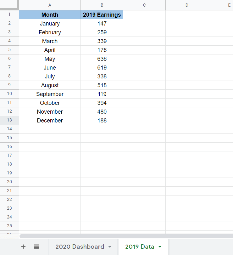
We also have another sheet with the monthly data from 2019.
We want to compare our current monthly earnings with data from the previous year. The final result should look something like this:

As you can see in the formula bar, this dashboard was completed through cell references. The data from both sheets followed the same monthly breakdown, so it was relatively simple to set up. We could have used a simple copy-paste here, but cell references allow you to make the data dynamic.
Let’s say that the sheet for 2019 is incomplete or needs updating in the future. If we simply use the copy-paste method, we’ll be left with old data in our dashboard. Cell references ensure that our data is always up-to-date.
This use case is just one way to use cell references in Google Sheets to link data in other tabs. We can use these cells independently, like in the example above, or we could use them as arguments for other functions or formulas.
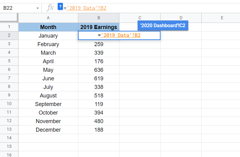
Cell references for data in other sheets follow a certain format. They follow the format
For example, we could reference cell C4 at the “Raw_Data” tab in other sheets using =Raw_Data!C4. If the sheet’s name includes a space, such as in “2019 Data”, the sheet name is surrounded by single quotes.
Now you know when pulling data from other sheets could be helpful. Let’s learn how to link the data ourselves in Google Sheets and later test it out with actual values.
A Real Example of Linking Data from a Different Tab
Let’s look at a real example of linking data from a different tab in your Google Sheets spreadsheet.
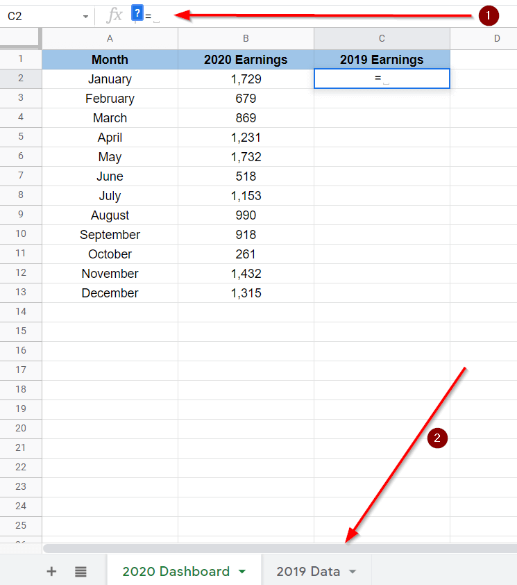
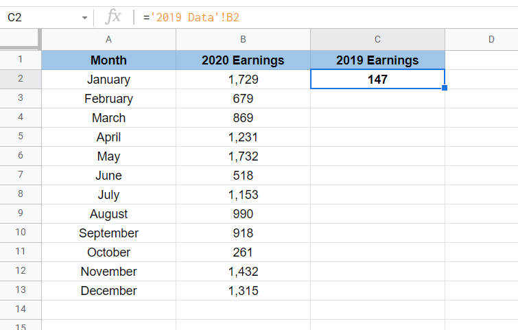
To get the values in Column C, we just need to use the following formula in cell C2:
='2019 Data'!B2
You can make your own copy of the spreadsheet above using the link attached below.
In this second example, we want to use data from the 2019 Data tab to get the percentage increase and decrease.

The formula we used is as follows:
= (B2 - '2019 Data'!B2)/'2019 Data'!B2
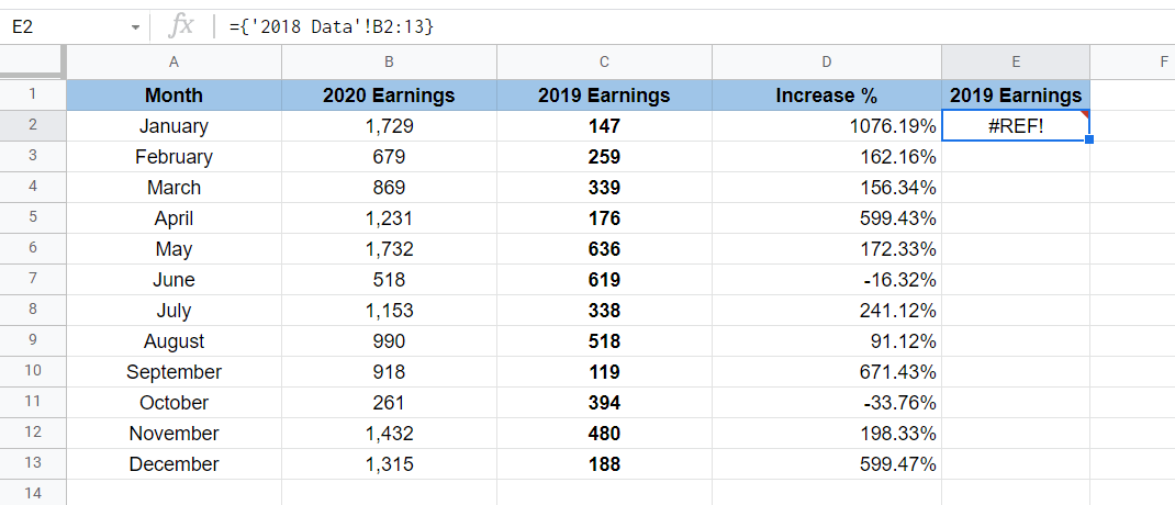
We can also link an entire range, row, or column. We just have to use curly braces around our cell reference. In the example below, we were able to get the same result in Column E, but we only needed to add a formula in one cell.
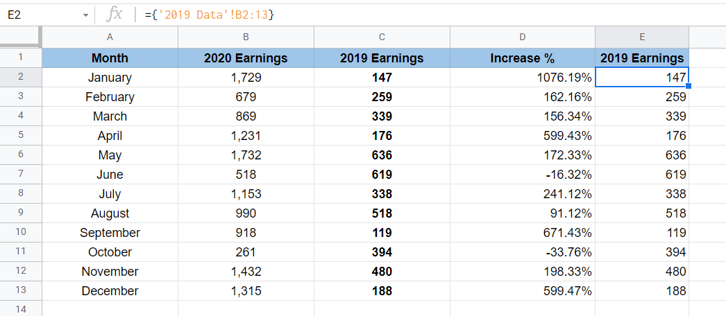
The formula we used to add an entire range is as follows:
={'2019 Data'!B2:13}
Let’s start linking the data ourselves. In the next section, we’ll go through the process step-by-step.
How to Link Data from a Different Tab in Google Sheets
This guide will show you how to link data from a different tab in Google Sheets using the example provided earlier.
Follow these simple steps to start linking data:
- First, select the cell which will hold the first cell reference. In this example, we’ll have to start at cell C2.
- Next, we just simply type the equal sign ‘=‘ to begin our formula. Afterward, we can click on the tab that contains our data.
- Next, select the cell we want to link. In this example, we want to get the corresponding January earnings from the previous year.
- Hit the Enter key on your keyboard to return the value in your original sheet.
- To fill out the rest of the column, we can drag the formula down. Select C2 and drag down the solid square found on the lower-right-hand side of the cell.

Frequently Asked Questions (FAQ)
- Why does my formula return an error?
Make sure that the cell reference is valid. If your sheet is not available in the current file, it will return a#REF!error. To ensure that cell references exist, you can always select the data or data range yourself when writing your formula.
- Can we use this method to get data from another worksheet?
The cell reference method only works for getting values within the same project or worksheet. We can use theIMPORTRANGEfunction to get ranges found in other projects. This function works by providing a URL to the second worksheet and a cell range to pull from.
That’s everything you need to know to start linking multiple tabs together in Google Sheets. This guide shows how easy it is to use cell references to make dynamic spreadsheets. Additionally, understanding how to link data from a different tab in Google Sheets makes handling redundant data more efficient.
You can now use this Google Sheets trick together with the various other Google Sheets formulas available to create great worksheets that fit your use case.
Make sure to subscribe to our newsletter made specifically for people interested in learning more about Google Sheets. Don’t miss out being the first to know about the latest in-depth guides and tutorials from us.