How To Link Multiple Spreadsheets in Google Sheets

Learning how to link multiple spreadsheets in Google Sheets is useful for instances wherein you need to present data located from other sheets.

In some cases, you’ll find it necessary to include data from other spreadsheets in your current spreadsheet. Although you can do this with the typical copy-paste approach, it’s not always the most efficient method as it only copies static data. This means that you only get to paste the exact data from the moment it was copied.

When working with advanced spreadsheets, there will be times when you need to import dynamic or real-time data. In such situations, it’s best to link multiple spreadsheets together. Thankfully, Google Sheets offers you a variety of ways to do this.

In this guide, we’ll cover the most efficient ways on how to link multiple spreadsheets in Google Sheets. We curated techniques that you can use for different occasions.

Let’s get started!

Referencing Another Sheet

The simplest way to link a specific worksheet to your current sheet is by writing a formula that references the name of the worksheet. This method is handy if you want to link multiple worksheets that belong on the same spreadsheet. To have a better grasp of this concept, let’s have a simple activity. Click the link below to generate a copy of our example spreadsheet.

Example 1

Our goal for this activity is to fill in the required data for the First Quarter Sales table of the main sheet. The data will come from the other sheets.

1. With the spreadsheet already open, notice that there are three sheets: Main Sheet, Canada, and Australia.
   
   
   
   For the first dataset (Canada), we’ll need to import the data from the Canada sheet. We will place the first record in cell A5 of the Main Sheet, so click this cell to select it.
   
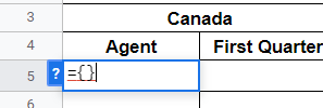
2. Now, Initiate the formula by typing in the equal sign ‘=’, followed by open and close curly brackets ‘{}’. The reason why we are including curly brackets in our formula is that we will be importing an array. In layman’s terms, an array is a set of data that consists of rows and columns.
   
   
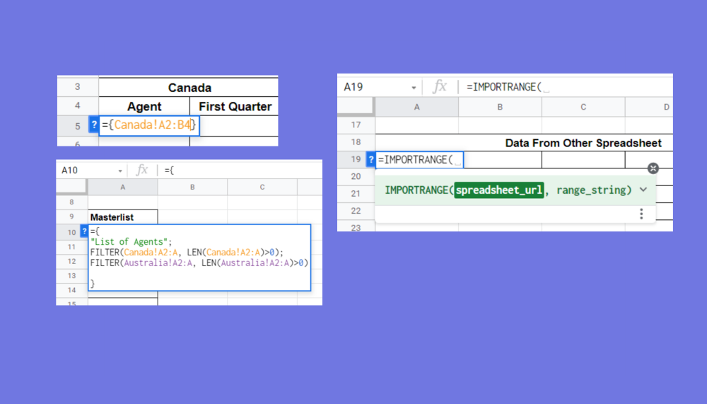
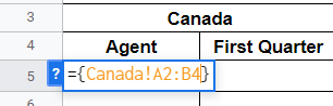
3. Inside the curly brackets, we need to define the parameters of our formula. Type in ‘Canada!A2:B4’.
   
   
   You’re probably wondering, what exactly does the formula do? It’s actually quite simple.
   
   The first part, ‘Canada!’ specifies the Sheet where we will import the data. In this case, it’s Canada. The next part, ‘A2:B4’, is specifically the cell range where we will acquire the data. We will use this formula to link or reference the sheet that contains the data we need to import.
4. Upon completing the formula, hit the Enter key on your keyboard. Your spreadsheet should already look like this.
   
   
   
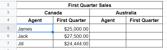
   Great! Now we have the first-quarter sales of the sales agents in Canada.
5. This time, try to import the next data set, which is the first-quarter sales of all the agents in Australia. In cell C5, type in the formula ‘={Australia!A2:B4}’. Afterward, press Enter. If your formula is correct, you should see this result on your spreadsheet:
   
   

Good job! Now you know how to reference a sheet to import its data. In the next section, you’ll learn another method of linking multiple spreadsheets on Google Sheets.

Using a User-Defined Formula to Link Multiple Sheets

Another technique for linking multiple sheets is to write a user-defined formula that utilizes the FILTER and LEN functions. This method is helpful in importing datasets from multiple sheets into one column. Let’s try this method for our next activity.

Example 2

For this activity, we will use the example spreadsheet we have earlier. Let’s say we want to generate a master list of all the sales agents from multiple sheets. To do so, we need to perform the following:

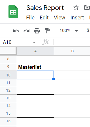
1. First, click on the cell where you need to import the data. In the example below, cell A10 is selected.
   
   
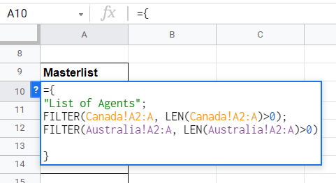
2. Next, double-click on the selected cell and type in this formula:
   
   ={
   “List of Agents”;
   FILTER(Canada!A2:A, LEN(Canada!A2:A)>0);
   FILTER(Australia!A2:A, LEN(Australia!A2:A)>0)
   }

   
   

   
   In a nutshell, here’s what the components of the formula do:
   • “List of Agents” – the first line indicates the column’s name to where the data will be placed.
   • FILTER(Canada!A2:A, LEN(Canada!A2:A)>0) – the second line uses the FILTER function to filter and return only the data within the entire column of A, beginning at cell A2 (A2:A) of the Canada sheet. In the case of the third line, we are trying to import data from the Australia sheet.
   • You’ll notice that the LEN function is used as the second parameter of the FILTER function. We used this parameter to ensure that we return only the data from the specified column with characters.
3. Once you’re done with the formula, press Enter, and your spreadsheet should now be similar to this.
   
   

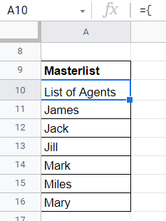
As you can see, with a user-defined formula, you can link multiple sheets to import their data into only one column.

Another scenario that you may encounter is linking into multiple sheets from different spreadsheets. What if the data you are trying to import is from another spreadsheet? If this is the case, the next method is your best bet.

Using the IMPORTRANGE Function to Import Data from Another Spreadsheet

If you’re not aware yet, the IMPORTRANGE function of Google Sheets is useful for linking multiple spreadsheets. Assuming that your data will come from an external source, specifically another spreadsheet, you can just use this simple function to retrieve the data you need.

Example 3

Apart from the example spreadsheet provided earlier, we’ll also need an additional spreadsheet that will serve as our external data source for this activity. Click on the link below to make a copy of our external data.

1. Before you can use the IMPORTRANGE function, there are two parameters that you need to consider: the URL of the spreadsheet, and the cell range of the data you want to import. In this case, open the External Data spreadsheet.
2. Our objective is to identify the cell range that contains the data we need to import. Let’s say that we need to import all the records of External Data, so the cell range we will need is A1:E4. Take note of this information as this will be the second parameter of our
   IMPORTRANGE function later on.
   
   
3. Next, copy the URL of External Data spreadsheet. This will be our first parameter.
   
   
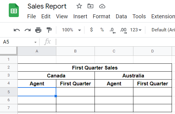
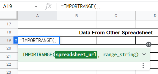
4. This time, open the Sales Report spreadsheet and look for the table with the heading ‘Data From Other Spreadsheet’.
   
   
5. At this point, double-click on the first empty cell, which is cell A19, and initiate the IMPORTRANGE function.
   
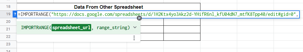
6. For the first parameter of IMPORTRANGE, paste the URL we have copied earlier and enclose it with double quotation marks.
   
   
7. This time, indicate cell A1:E4 for the second parameter of IMPORTRANGE. Like the first parameter, make sure to enclose it also with double quotation marks.
   
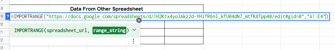
8. Finally, press Enter, and your spreadsheet should already be like this.
   
   

Perfect! Now you know how to use the IMPORTRANGE function to link another spreadsheet in your current spreadsheet.

There you have it! We just showed you different techniques on how to link multiple spreadsheets in Google Sheets. Check out other useful functions in Google Sheets to make your work more efficient.

Subscribe to our newsletter to receive more useful articles like this one about Google Sheets.

Get emails from us about Google Sheets.

Our goal this year is to create lots of rich, bite-sized tutorials for Google Sheets users like you. If you liked this one, you'll love what we are working on! Readers receive ✨ early access ✨ to new content.

Subscribe