How to Auto-Populate Dates Between Two Given Dates in Google Sheets

To auto-populate dates between two given dates in Google Sheets is useful if you have a start date and an end date and you want to fill all the dates between these two dates in a column.

Auto-populating means filling a column automatically with the values between two given values. You can auto-populate both numbers and dates to make your work faster and easier.

Let’s take an example.

Say we have a start date and an end date. We want to expand the dates between these two given dates in our spreadsheet and see the days one by one in a column.

So how do we do that?

Simple. We can use the SEQUENCE function and some additional functions, ARRAYFORMULA and TO_DATE, to do this automatically.

In this guide, I’ll show you how you can do this with one single formula.

Let’s dive right in. 🤜

The Anatomy of the Auto-Populating Functions

We’re showing the combination of three different functions to auto-populate dates between two given dates in Google Sheets.

The SEQUENCE Function

The SEQUENCE function is used to return an array of sequential numbers.

The syntax (the way we write) the SEQUENCE function is the following:

=SEQUENCE (rows, columns, start, step)

The variables of the function are:

• rows means the number of rows we want in the sequence,
• columns means the number of columns where we want to expand the sequence,
• start is the first value of the sequence,
• step indicates the difference between two values of the sequence. Its default value is 1.

To understand how to use exactly the SEQUENCE function in Google Sheets, check our article that explains it in details.

Since Google Sheets treats every date as integer numbers in the background, we can use the SEQUENCE function with dates as well.

The TO_DATE Function

The TO_DATE function converts a given number to date.

Its syntax is as follows:

=TO_DATE(value)

It takes one cell with a number (as the value variable) and converts it to date.

Although we could convert our numbers to dates by formatting them in the menu (Format > Number > Date), using this function instead saves a lot of time when there are many rows.

The ARRAYFORMULA Function

The ARRAYFORMULA function in Google Sheets applies a formula to an entire column in Google Sheets.

It’s used when we have a function that normally works on one cell, but we want to use it on a whole range of cells. For example, the TO_DATE function works with one cell, but we want to use it on a whole column.

The syntax of the ARRAYFORMULA function is:

=ARRAYFORMULA(array_formula)

The array_formula variable is the function that we want to wrap in an ARRAYFORMULA. We can use any function in the ARRAYFORMULA function that can be applied to a whole range of cells.

Read more about the ARRAYFORMULA function in our article.

So, after having gained some insights into the anatomy of these functions, let’s use them in a real-life example.

A Real Example to Auto-Populate Dates Between Two Given Dates

Have a look at the example below to see how to auto-populate dates between two given dates in Google Sheets.

The picture below shows the expected result. It contains the start date and the end date, together with the auto-populated list of dates.

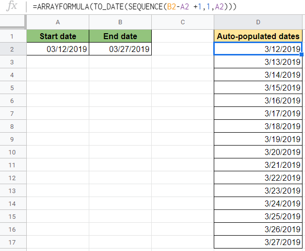
The function we used here is as follows:

=ARRAYFORMULA(TO_DATE(SEQUENCE(B1- A1 +1,1,A1)))

Let’s break this down to understand what each of the parts means:

• First, look at the most inner function of this formula. We used the SEQUENCE function to create the array of sequential numbers. Remember that every date is a number in the background, that’s what we used to calculate the rows variable.
• The rows variable of the SEQUENCE function is the number of rows we want in our sequence. Thus, it’s the difference between the start and end date, plus one because we want to include the end date itself too. We used the cell references of the start and end dates, subtracted them and added 1 to the result. So, the rows variable is B1 – A1 + 1.
• Then, the columns variable is 1 because we only need one column.
• The start variable is the start date which is in cell A1.
• Then, we used the TO_DATE function to convert the numbers to dates.
• Finally, we wrapped the whole function in the ARRAYFORMULA function to ensure that the TO_DATE function is applied to every cell of the result of the SEQUENCE function.

As a result, we got a list with auto-populated dates between the start date and the end date.

It’s simple, right?

Feel free to make a copy of the spreadsheet using the link I have attached below and try it for yourself:

How to Auto-Populate Dates Between Two Given Dates in Google Sheets

Let’s see how can you auto-populate dates between two given dates in Google Sheets step-by-step.

1. To start, select the cell where you want to have the first date of the auto-populated range. Make sure to have sufficient empty area below this cell, because the function will expand down the entire column.

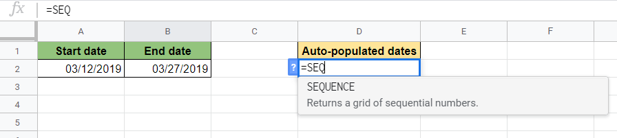
2. Then, enter the equal sign ‘=’ to begin the formula and then followed by the name of the SEQUENCE function. For this guide, I will be typing it in cell D2.

3. After the opening bracket ‘(‘ of the SEQUENCE function, add the first variable, rows. To define how many rows you want in your sequence, subtract the start date from the end date. For this guide, I will be selecting the cells B2 and A2 to calculate this difference.

4. Then, add 1 to this number if you want to include the end date as well. Otherwise, you would only auto-populate the dates until the day before the end date. Put a comma after each variable of the function.

5. After that, add the columns variable which is 1 in this example.

6. To finish the SEQUENCE function, add the start variable that is the first number (date) of your sequence. In the example, I will be selecting the cell A2 that has my start date.

7. Great! This formula would already return a sequence of numbers that can be formatted as dates. However, I’m showing a way to include the formatting in the formula itself. Close the brackets of the SEQUENCE function and move your cursor after the equal sign at the beginning. After that, type the name of the TO_DATE function here.

8. There is one more thing left. Converting the single-cell result of the TO_DATE function into an array. Therefore, close the brackets of the TO_DATE function as well and go back to the equal sign again. Wrap the whole formula in an ARRAYFORMULA function.

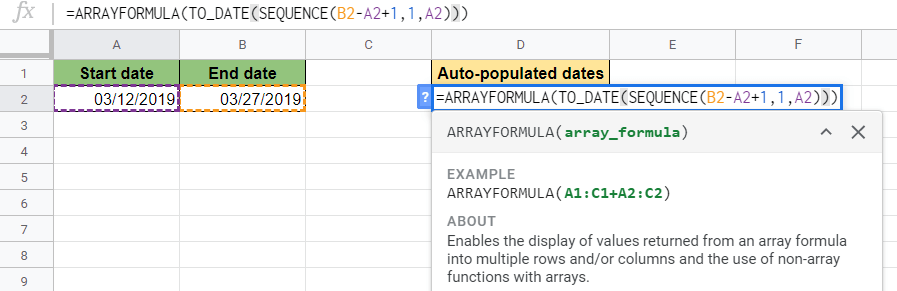
9. Finally, hit your Enter key to see the whole sequence of auto-populated dates.

That’s it! This is how you auto-populate dates between two given dates in Google Sheets using the SEQUENCE, TO_DATE and ARRAYFORMULA functions. 👏🏆

Now you can use it together with the other numerous Google Sheets formulas to create even more effective formulas. 🙂

Get emails from us about Google Sheets.

Our goal this year is to create lots of rich, bite-sized tutorials for Google Sheets users like you. If you liked this one, you'll love what we are working on! Readers receive ✨ early access ✨ to new content. There will be no spam and you can unsubscribe at any time.

Subscribe