How to Use VAR Function in Google Sheets

The VAR function in Google Sheets is useful to calculate the variance of a dataset to measure the dispersion in a group of numbers.

The variance is an essential statistical function that measures how far a set of numbers in an entire population are spread out from their average value.

Let’s take an example.

Say we have a group of people of different ages. 👶👴

The average (mean) age of the group is an important value, but we also want to know how much spread there is around that average.

If the average age in a group is 35, it could be the case that every person in the group is exactly 35 years old. Or it could be that half the people were exactly 0 years old and the other half was exactly 70 years old. Or anything else in between.

The average age in all these cases is 35.

Thus, we use the variance to measure how dispersed the ages of the people are varying from the average age. If this number is greater, then it means that the values are more spread out.

So how do we do that?

1. Count the average of the numbers (add all the values and divide it by the number of values).
2. Then for each number, subtract the average and square the result. By squaring, you avoid negative numbers.
3. After that, work out the average of those squared differences, but instead of dividing by the number of values, divide it by the number of values minus one. The result is the variance.

In Google Sheets, you don’t need to calculate this manually, but you can use the VAR function to get the variance in some easy steps. The function calculates it all automatically.

Now, let’s dive right into real examples to see how to use VAR function in Google Sheets.

The Anatomy of the VAR Function

The syntax (the way we write) the VAR function is as follows:

=VAR(value1, [value2, ...])

Let’s break this down and understand what each of these terms means:

• = the equal sign is how we start every function in Google Sheets.
• VAR is our function. We will have to add the values into it for it to work.
• value1 is the first value or range of the sample, and it is a required field.
• value2 , value3 , … are additional values or ranges to include in the calculation. Their use is optional.

As you can see, you can use either values or ranges to count the variance. This means that the arguments (value1 , value2, and so on) can be numbers, cell references, or ranges of cell references.

Let’s see how does this works when you write your function.

• If you use direct numeric values in the function, then it calculates the variance of these actual numbers:

=VAR(1, 3, 6, 8, 11, 18)

• In case you want to include the cell references of the numbers, you can do the following, putting several cell references as values:

=VAR(A4, B3, D10, H1)

• Nevertheless, it’s more common to use references to ranges of the sheet to calculate the variance of the numbers in our ranges. You can write such a function with one single range, and the function will include all the numbers in this range:

=VAR(A1:A100)

• One range counts as one value in the function. Therefore you can even add more than one ranges to the function if your values are located in different parts of the sheet:

=VAR(A1:A20, C4:C11, F10:F30)

⚠️ Now a few notes when you write a VAR function

1. If the total sum of numbers supplied to the function is not at least two, VAR will return the #DIV/0!​ error.
2. Text values and other non-numeric values will be ignored by the function, so you don’t have to manually exclude these cells.
3. The VAR function will return an error if all of the value arguments are text. You can use the VARA function to calculate variance while interpreting text values as 0.
4. The VAR function takes the sum of the squares of each value’s deviation from the mean and divides by the number of such values minus one. This is different from the calculation of variance across an entire population because the population variance divides by the size of the dataset without subtracting one. To calculate the variance based on an entire population, use the VARP function.
5. Another widely used statistical function is the standard deviation. It’s closely related to the variance because it is computed as the square root of it. You can calculate the population standard deviation in Google Sheets using the STDEVP function.

A Real Example of Using VAR Function

Take a look at the example below to see how the VAR function is used in Google Sheets.

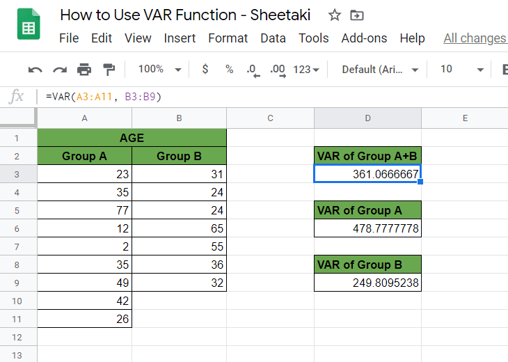
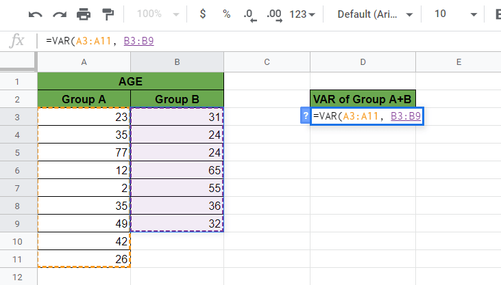
The example above shows how we used the VAR function to calculate the variance of the ages of people. The people are separated into two groups called Group A and Group B. We calculated both the variance of each group and also the variance of all of them combined.

The function to calculate the variance of Group A is:

=VAR(A3:A11)

Secondly, the variance of Group B is calculated with the following function:

=VAR(B3:B9)

But let’s look further into how we wrote the function when we included all the numbers in the calculation.

The function to calculate the variance of Group A and Group B combined is as follows:

=VAR(A3:A11, B3:B9)

Here’s what this example does:

• Firstly, we made a cell active. This is where we will write our VAR formula. For this guide, we selected cell D3.
• Next, we started off our formula with an equal sign, followed by our function, VAR.
• After that, we added our values into it. Since we have some of the numbers in column A, we referenced them as one range (A3:A11).
• Then, we have the rest of the numbers in column B. At this point, we added this range (B3:B9) as the second value of the function.
• You can see the result 361.0666667 in cell D3, which is the variance. This number represents how diverse are the ages of the list from their average value.

See how simple that is! The VAR function performs all the mathematical calculations automatically.

Go ahead and give it a shot! 😀 Using the link I have attached below you can make a copy of the spreadsheet:

How to Use VAR Function in Google Sheets

Let’s see how to write your own VAR function in Google Sheets step-by-step.

1. To start, click on the cell where you want to show your result to make it the active cell. For this guide, I will be selecting D3, where I calculated the variance of all the numbers of both Group A and Group B.

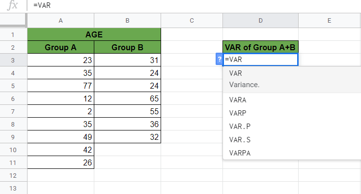
2. Next, type the equal sign ‘=’ to begin the function and then followed by the name of the function which is ‘var‘ (or VAR, whichever works).

3. Now you should see that the auto-suggest box will pop-up with the name of the functions that start with VAR. There are more of them, so make sure to select the right one!

4. After the opening bracket ‘(‘, you have to add the values. Remember that you can add more than one ranges containing the values. Firstly, highlight the range of Group A with your mouse. The range is A3:A11 in my example.

5. After that, add a comma to separate the values and highlight the second range, including the numbers of Group B. The range is B3:B9 in my example.

6. Finally, if you added all the ranges you wanted to include, hit the Enter key to close the brackets and get the result. Great! You can see the variance of the data set in cell D3.

That’s it! You can now use the VAR function together with the other numerous Google Sheets formulas to create even more powerful formulas that can make your life much easier. 🙂

Get emails from us about Google Sheets.

Our goal this year is to create lots of rich, bite-sized tutorials for Google Sheets users like you. If you liked this one, you'll love what we are working on! Readers receive ✨ early access ✨ to new content.

Subscribe