How to Use MODE Function in Google Sheets

The MODE function in Google Sheets is useful when you want to find the most frequently occurring value in a dataset. 

The function analyzes your data and identifies the value that appears the most.

There are a few things to remember when using the MODE function:

• The MODE function can only be used on numbers, dates, or times. 
• If there are two (2) or more values that appear most, the MODE function will show the first value it finds on the database.

Here’s an example.

A chef opens a bakery that sells cheesecakes in jars. At the end of a successful first week, he wants to know which sales agent sold the most number of jars so that he can reward them. He also wants to know which day had the most sales. 

Instead of sorting or combing through his records day by day, he can use the MODE function to find the information straightaway. 

The process is simple and effective. ✅

That’s one situation of the practical application of the MODE function, but there are many others. Its biggest advantage is that it’s applicable to any data, both nominal and numerical. As the function can only be applied to numbers, dates, or times, you just need to make sure each nominal value is assigned a numbered ID. 

Whatever purpose you have for using the MODE function, it will simplify your task of finding the most common value in a dataset.

Now, let’s dive into an illustrated guide to really get a better picture of how and when to use the MODE function in Google Sheets.

The Anatomy of the MODE Function

So the syntax (the way we write) of the MODE function is as follows:

=MODE(value1, [value2, …])

Let’s dissect this and understand what each of these terms means:

• = the equal sign is how we start any function in Google Sheets. Without the equal sign, it won’t become a formula but remain as plain text.
• MODE() this is the MODE function. It will analyze your given dataset and return the mode, which is the value that is most frequently occurring. If there would ever be more than one mode, the formula will return the first value it finds on the dataset. 
• value refers to the data you want to calculate the mode for. At least one value is required for the function to work. The dataset also needs to be in the form of numbers, dates, or times. It won’t work on nominal values or text. Otherwise, it will return an #N/A result. You can have as many values as you want to consider. There are no limits to the size of the dataset. Google Sheets supports an arbitrary number of arguments for this function.

A Real Example of Using MODE Function in Google Sheets

Let’s go over the example below to see how MODE functions are used in Google Sheets.

The chef recorded all the sales for the week under the table SALES RECORDS. He also assigned each of his sales agents a numerical ID. He wants to know which agent sold the most cheesecakes, and which date had the most sales. 

One way to get the information he wants is to sort the SALES RECORDS according to the AGENT ID instead of the DATE. Then he can manually count how many times each agent ID appears, but that’s too much work. He can bypass that entire process by using the MODE function. 

Look at the yellow tables. Using the MODE function on the Agent ID, he was able to identify that Agent ID 101 appeared the most number of times. In this context, this means Agent 101 sold the most jars during the week. Likewise, using the MODE function on the dates, he was able to identify that the day with the most sales was January 1, 2021. 

Feel free to make a copy of this spreadsheet through the link below.

If you look closely at the table, you will actually notice that there are two values that appear most. Both Agent ID 101 and 104 appear 8 times on the table, but the result of the MODE function is 101. This is because the MODE function only returns the first value. In this case, 101 appears on the table before 104. 

Fortunately, this situation has an easy solution. Instead of the MODE function, you can use the MODE.MULT function. If there are two or more modes in a database, the MODE.MULT function will return all of them. 

To learn more about the MODE.MULT function, click on this link to go to our tutorial.

Great! Let’s begin writing our own MODE function in Google Sheets.

How to Use MODE Function in Google Sheets

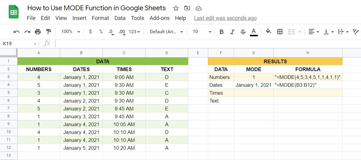
1. First, prepare the data you want to use. Make sure that they are in a number, date, or time format. To illustrate what happens when the data is a text, we also included textual data.

2. Next, click on the cell you want the result to appear in. Any cell will do. In this example, we’re using cell G3. Type the equal sign ‘=‘ to begin the function. Follow that by the name of the function which is ‘mode‘ (or ‘MODE‘, either one works). Once you’ve done that, you can proceed to the next step.

3. You should find that the auto-suggest box appears with the names of the functions that all start with MODE. You’ll see our two variants, MODE.SNGL and MODE.MULTfunctions, in the list too. We’ll take up MODE.SNGL and MODE.MULT in another tutorial. For now, select MODEby pressing the Tab or Enter keys on your keyboard. A pop-up box will appear below the cell you’re working on. This is a guide from Google Sheets that tells you more about the function you’re using. If you want to minimize it, just click on this ^ symbol on the upper right of the box beside the x.

4. Now that you have the start of your MODE function, let’s put in the values. You can choose to put a set of numbers (as shown below), a range of cells, or both. Once you have all the values you need, end the function with a close parenthesis.

5. Now, hit your Enter key on your keyboard. You should be able to see the result in the cell you used. For this example, the mode of the Numbers data is 1.

6. Let’s try another one! This time, let’s find which of the Dates appear the most times in the data. For efficiency, select a range of cells to input the values. To do that, click the first cell and drag your mouse to the last cell in the range. In this example, the selected cell references are B3:B12.

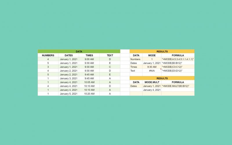
7. Press the Enter key on your keyboard to show the result. For this illustration, the mode of the Dates data is January 1, 2021.

8. Remember to have your data in a number, date, or time format. Otherwise, the function will result in an #N/A. See the mode for TEXT in the image below as a reference.

That ends our tutorial. You can now use the MODE function in Google Sheets to extract information from a vast amount of data more efficiently and effectively. 

If you have any questions left unanswered, refer to the FAQs down below. Hopefully, you’ll find the answers you need there. 

Frequently Asked Questions (FAQ)

1. How can I get more than one result from the MODE function?

   There will definitely be times when a dataset will have more than one mode. In such cases, use the MODE.MULT function instead. The MODE.MULT function will show all the values that appear the most in the dataset, and not just one. To learn how to use the MODE.MULT function, be sure to subscribe so that you’ll be notified when it becomes available.

2. What do I do when the results I get are #N/A?

   This happens when you’re trying to find the mode in a nominal or textual data format. You can certainly use the mode function on nominal data, but not directly. You will need to convert your textual data into a numerical format. That means you assign each textual data with a unique number. You will then use those numbers as the values in your MODE function. 

And that’s it! You can now use the MODE function in Google Sheets. Combine it with other functions, and you’ll create even more powerful and efficient formulas that’ll make your life easier. 🙂

Get emails from us about Google Sheets.

Our goal this year is to create lots of rich, bite-sized tutorials for Google Sheets users like you. If you liked this one, you'll love what we are working on! Readers receive ✨ early access ✨ to new content.

Subscribe