The MODE.MULT function in Google Sheets is useful when you want to find one or more values that most frequently occur in a dataset.
The MODE.MULT function is a variation of the MODE function that gives one or more results, depending on the data.
Table of Contents
There are a few things to remember when using the MODE.MULT function:
- The
MODE.MULTfunction can only be used on numbers, dates, or times. - The
MODE.MULTfunction shows all the values that appear most in a dataset. This means that you need to leave empty cells below the cell with the function for the results to appear. Otherwise, it will result in a #REF! error.
Here’s an example.
A chef opens a business that sells cheesecakes in jars. At the end of his first week, he wants to award the sales agent/s with the most sales. He also wants to know on which days they had the most sales.
Instead of sorting through his records and manually counting the sales per agent, he can use the MODE.MULT function to find the information straightaway.
The process is simple and effective. ✅
That’s one situation where the MODE.MULT function can be useful, and there are many others. Its biggest advantage is that it can be used on any data, both nominal and numerical. Just remember that the function can only be used on numbers, dates, or times. This means that in order to find the mode of nominal data, you must first assign each data a unique numeric ID. You will then use the MODE.MULT function on the number ID.
However you want to use the MODE.MULT function, it will definitely save you time and effort.
Let’s dive into this guide to really get a better picture of when and how to use the MODE.MULT function in Google Sheets.
The Anatomy of the MODE.MULT Function
So the syntax (the way we write) of the MODE.MULT function is as follows:
=MODE.MULT(value1, [value2, …])
Let’s go through the elements one by one to understand what they mean:
=the equal sign is how we start any function in Google Sheets. Without the equal sign, The formula won’t work but remain as plain text.MODE.MULT() this is theMODE.MULTfunction. It will analyze your given dataset and return all possible modes, which is a value that most frequently occurs in a dataset. There can be more than one mode in a dataset, and this function will return all of them.Valuerefers to the dataset you want to calculate the modes for. The function requires at least one value and needs to be in the form of numbers, dates, or times. Nominal or textual values will result in a #N/A error. You can have as many values as you want to consider, as there are no limits to the size of the dataset. Google Sheets supports an arbitrary number of arguments for this function.
A Real Example of Using MODE.MULT Function
Let’s go through this example below to see how MODE.MULT function is used in Google Sheets.

The SALES RECORDS is where the chef takes note of each agent’s sales. He wants to know which of his agents sold the most number of cheesecakes, and on what dates. Sorting the SALES RECORDS according to the AGENT ID, then manually counting how many times each agent ID appears, is one way to do it. But that’s too much work, and it rearranges the dataset itself. Instead, he can use the MODE.MULT function which will give him more accurate results.
Now, the agents’ names are nominal values. They aren’t numbers, dates, or times. So for the MODE.MULT function to work, the chef assigns each sales agent a unique number. In this example, it’s called the AGENT ID.
Refer to the yellow tables. Using the MODE.MULT function on the Agent ID, the chef is able to identify that Agent IDs 101 and 104 (Frodo Baggins and Peregrin Took, respectively) sold the most jars during the week. Likewise, by using the MODE.MULT function on the dates, he is able to identify that the days with the most sales were January 1, 2021, and January 2, 2021.
Feel free to make a copy of this spreadsheet through the link below.
Had the chef used only the MODE function, the results would have been different. The MODE function only returns the first mode it finds on the dataset. So in this situation, the MODE function would have only shown Agent 101 and January 1, 2021. It would have left out Agent 104 and January 2, 2021.
If you want to learn more about the MODE function, check out our guide through this link here!
Great! Let’s begin writing our own MODE.MULT function in Google Sheets.
How to Use MODE.MULT Function in Google Sheets
- Firstly, prepare the dataset that you want to use. Remember to put them in a number, date, or time format. We also included textual data to illustrate the effects of the
MODE.MULTfunction on texts.

- Next, click on the cell you want to use. Any cell will do. Remember that the
MODE.MULTfunction can return more than one result. If the cells below contain data, the function will return a #REF! error. So make sure that the cells below the one with the function are empty.
- Type the equal sign ‘=‘ to begin the function. Follow that by the name of the function which is ‘
mode.mult‘ (or ‘MODE.MULT‘, either will work). Once you have the function, it’s time to add the values. Refer to the next step.

- Now, we input the values. You can input a set of numbers (as shown in the image below), a range of cells, or both. We’ll cover using a range of cells as values in a later step. Once all the values have been inputted, end the function with a close parenthesis.

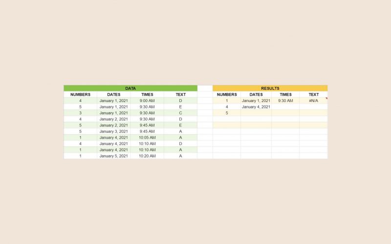
- Finally, it’s time to see the results. Hit the Enter key on your keyboard. You will see that the results will appear in the cell you used and the cells below it. The results show that 1, 4, and 5 appear the most frequently on the dataset. If your function results in a #REF! Error, the cells below the function contain data, so make sure they’re clear of any data.

- Let’s have another example! Let’s use the
MODE.MULTfunction on dates. For efficiency, let’s select a range of cells to input as the values of the function. Click on the first cell of the range and drag your mouse to the last cell. The value should show something similar to (B3:B12).

- Get the results by pressing the Enter key on your keyboard. In this example, the modes of the Dates data are January 1, 2021, and January 4, 2021.

- Remember that for data to be considered valid values in the function, they must be in a number, date, or time format. The function will result in an #N/A error otherwise. See the results under TEXT in the image below.

That ends our tutorial on how to use the MODE.MULT function in Google Sheets. You can now calculate the modes of a vast amount of data more efficiently and effectively.
Frequently Asked Questions (FAQ)
-
Why does my function result in a #REF! error?
The
MODE.MULTfunction can generate more than one result and lists them down below the cell with the formula. You will get a #REF! result if the cells below theMODE.MULTfunction are occupied. Take this example. To resolve this, just make sure the cells below theMODE.MULTfunction are empty.

-
What do I do when the results I get are #N/A?
You get a #N/A error when the values in your function are in a nominal or textual data format. While you can certainly use the
MODE.MULTfunction on nominal data, You will first need to convert your textual data into a numerical format. That means you assign each textual data with a unique number ID. You can then use the unique numbers as values in yourMODE.MULTfunction.
And that’s it! You have just added the MODE.MULT function into your repertoire of Google Sheets functions. Combine all you’ve learned, and you’ll create even more powerful and efficient formulas that will make your life easier and save you more time. 🙂


