The NETWORKDAYS function in Google Sheets is useful if you want to know how many working days there are between two dates.
The function returns the number of days between two given dates, excluding weekends and holidays listed within the Google Sheets.
Table of Contents
Let’s take an example:
You have assignments due for each subject you take in school. You would like to know how many days are available for you to complete the assignments.
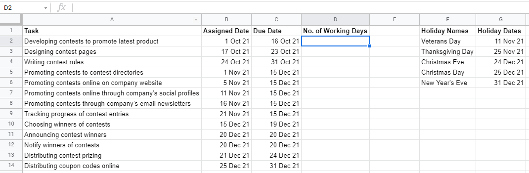
Simply list down all the assignments in Google Sheet with the start and end dates. Then use the NETWORKDAYS function to check the days available. Here is how it looks like on Google Sheets:
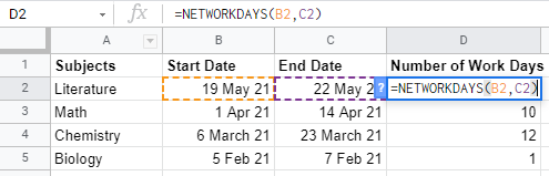
Now you can plan a timetable to work on the weekdays and chill out on the weekends! 🙌✨
The Anatomy of the NETWORKDAYS Function
The way we write the NETWORKDAYS function is:
=NETWORKDAYS(start_date,end_date,[holidays])
Let us help you understand the context of the function:
- The equal sign
=is how we start any function in Google Sheets. NETWORKDAYS()is our function. We need to add two attributes, namely thestart_dateandend_date, to make it work correctly. We can also add the[holidays]into the formula to exclude those dates.- The
start_dateis the start date of the period from which to calculate the number of net working days. - The
end_dateis the end date of the period from which to calculate the number of net working days. - The
[holidays]is a range of dates containing the dates that are considered holidays. This is optional.
Let’s take note that:
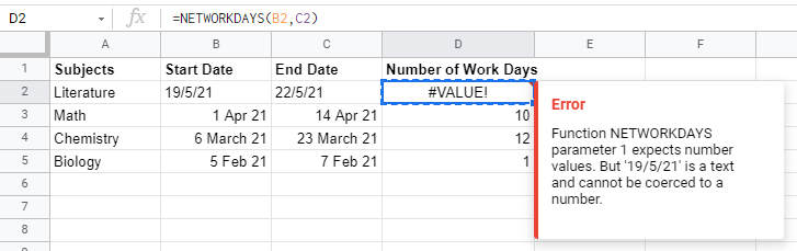
The dates used in this formula need to be serial dates, not text dates. If not, the function could not understand the attributes being input.
For example:
A Real Life Example of Using NETWORKDAYS Function
Example 1:
Let’s use a real-life situation to utilize the NETWORKDAYS function to see how the function is used in Google Sheets.
This example shows how you can create a timeline for actions/ tasks to complete for a particular project or campaign. By using the NETWORKDAYS function, you can exclude non-working days like the weekends and holidays to accurately depict your timeline. 👌
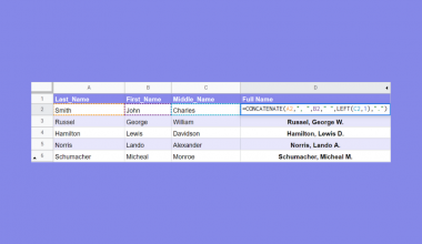
How to Use NETWORKDAYS Function in Google Sheets
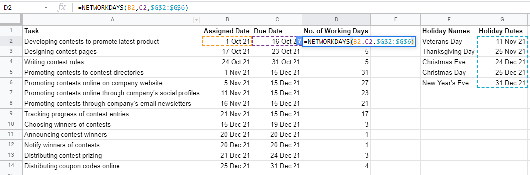
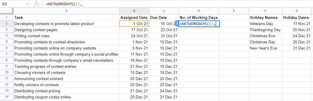
- Simply click on the cell that you want to write down your function at. In this example, it will be D2.
- Begin your function with an equal sign
=, followed by the name of the function,NETWORKDAYS. Don’t forget to add an open parenthesis(

- We will then select cell B2, as this is the
start_dateof the task. Furthermore, we need to add a comma,to separate thestart_datefrom our next attribute, theend_date.
- Next, we will select cell C2, as this is our
end_date.

- Then, we will add another comma
,to separate theend_datefrom the[holidays]. To include the[holidays], simply select the range of dates listed in the Google Sheets. We end the formula by closing it with a parenthesis).
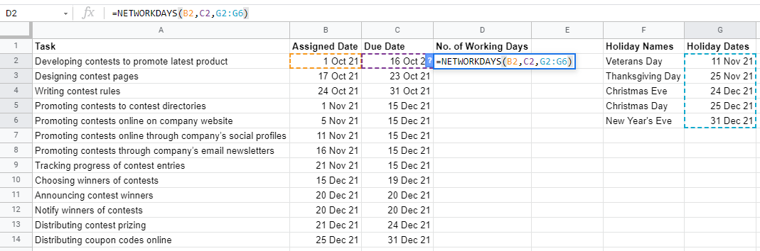
Our final formula would look like this:
=NETWORKDAYS(B2,C2,G2:G6)
- After the following steps, your input should look like this.

Example 2:
Let us show you another scenario where you can utilize the NETWORKDAYS function in other areas of your business.

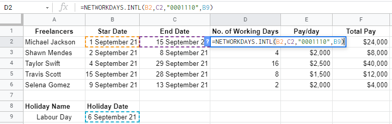
Payroll can get pretty hectic at the end of each month if you have many workers 💆. By using the NETWORKDAYS function, you can calculate the number of working days for each freelancer excluding the weekends and holidays within the month.
Apply the same steps from above and you will get the number of working days.

After you get the number of working days, multiply it with the rate per day charged. Now you get the total pay for each freelancer and avoid paying more than they required! As simple as that!
A Step-up From NETWORKDAYS Function
However, let’s say your company’s “weekends” do not fall on the traditional “Saturday” or “Sunday”. If that’s the case, you can still use the NETWORKDAYS.INTL function.
The NETWORKDAYS.INTL function is a step up from the NETWORKDAYS function. By including the “INTL” as an additional attribute, it represents which days of the week are considered weekends to you!
The formula will look like this:
=NETWORKDAYS.INTL(start_date,end_date,[weekend],[holidays])
Similar to the [holidays] attribute, [weekend] is optional as well.
Let’s take note that:
There are two methods to input [weekend] into the formula:
- String Method: weekends can be specified using seven
0’s and1’s, where the first number in the set represents Monday and the last number is for Sunday. A0means that the day is a weekday and a1means that the day is a weekend. For example,0000011would mean Saturday and Sunday are weekends. - Number Method: instead of using the string method, a single number can be used. Here are the number representations:

Let’s take an example:
We shall use Example 2 as an example, but instead of the weekends being Saturday and Sunday, the Company’s policy shows that the weekends are on Fridays and Saturdays.
Easy! We will use NETWORKDAYS.INTL function to modify the Fridays and Saturdays to represent weekends.
As shown in the table above, to represent Fridays and Saturdays as the weekend, we will use the number 7.
This is how the formula would look like for NETWORKDAYS.INTL function using the number method in Google Sheets:

We can also use the string method. For example, if the company offers Thursdays, Fridays, and Saturdays as weekends, the number method can no longer be applied. No worries! Let’s use the string method in the formula to calculate the working days.
To make Thursdays, Fridays, and Saturdays to represent weekends, the string method would be 0001110. To avoid confusion, here is a table to make things easier:

This is how the formula would look like for NETWORKDAYS.INTL function using the string method in Google Sheets:
You may make a copy of the spreadsheet using the link attached below and try it for yourself:
There you go!
There are many ways to calculate the days between two given dates, and for different scenarios, a different function may be more suitable. Click here to learn more!