The NPER function in Google Sheets is useful if you want to calculate the number of payment periods for a loan or investment, where the periodic payment and interest rate are constant.
Table of Contents
The NPER function does this simply by supplying the given details such as the rate, payment amount, present value, future value, and determining whether payments are due at the end (‘0’) or beginning (‘1’) of each period.
Let’s take an example to understand how the NPER function works.
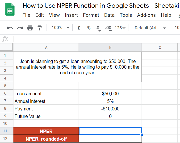
Say we are planning to get a loan amounting to $50,000. The annual interest rate is 5%. We are willing to pay $10,000 at the end of each year.
So how do we do that?
Easy. We can use our NPER function to calculate how many payment periods are needed. We will list down the given details for easier substitution. The rate is 5%, we are willing to pay $10,000, and the total loan amount is $50,000. As we work on the formula, we will now substitute it with the numbers given. The NPER function will provide us with a result of 5.89631286. Since we are talking about the number of years, we will then round it off to get an answer of 6 years.
See how easy that is?
Let’s dive right into real-business examples where we will deal with actual values and textual strings and how we can write our NPER function in Google Sheets to compute those data.
The Anatomy of the NPER Function
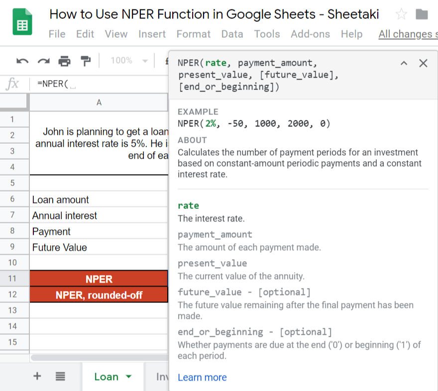
So the syntax (or the way we write) the NPER function is as follows:
=NPER(rate, payment_amount, present_value, [future_value], [end_or_beginning])
It can be overwhelming at this point, but let’s break it down to pieces to understand better what each term mean:
=the equal sign is just how we start any function in Google SheetsNPER()this is ourNPERfunction which we enclose with all the corresponding attributes,rate,payment_amount,present_value,future_valueandend_or_beginningwithin parenthesis.rateis the annual/yearly interest rate.payment_amountis the amount of each (periodic) payment (PMT).present_valueis the present value (PV) (sum of all the payments).future_valueis the future value (FV) or the cash balance that you want to attain after the final payment. This is optional and defaults to 0.end_or_beginningis whether the payment is due at the end or beginning of each period. This is also optional. The default value is 0 (payment at the end of the period). If beginning, we use 1.
⚠️ Now a few notes before using the NPER Function in Google Sheets.
- The rate that we will supply in the formula should be the annual or yearly
rate. If the requiredNPERis quarterly, then simply divide therateby 4 to get the quarterlyrate. If the requiredNPERis annually, but therategiven is quarterly, just multiply it by 4 to get an annualrate. The same when we are dealing with monthly calculations, replace 4 to 12.

- The
payment_amountmust be shown as negative because it’s outgoing.
Now it may look confusing, but rest assured, we will go through every step and subsequently practice applying it.
A Real Example of Using NPER Function
Take a look at our example below to see how the NPER function is used in Google Sheets.

As you can see in our example above, we used the NPER function to find how many payment periods does John need for a $50,000 loan with 5% interest. We got an answer of 5.89631286, and we rounded it off to get 6. The function is as follows:
=NPER(5%,-10000,50000,0)
Here’s what this example does:
- We have actively selected cell B11, and we want to use the
NPERfunction to calculate the payment periods. - Then, we identified all the given details: $50,000 is the loan, 5% is the interest, and $10,000 is the payment.
- Using the pop-up message as a guide, we supplied the needed values as identified in the previous step.
- Lastly, we closed our formula and hit on the Enter key.
Another example that the NPER function is handy is when we make an investment, and we want to know the total number of periods required to reach that specific goal:

As you can see in our example above, we used the NPER function to calculate the total number of the period required for John to reach his goal. We got an answer of 23.73716556, and we rounded it off to get 24. The function is as follows:
=NPER(5%/12,-2000,0,50000,1)
Here’s what this example does:
- We have actively selected cell B12, and we want to use the
NPERfunction to calculate the number of periods. - Then, we identified all the given details: $50,000 is future value, 5% is the interest, and $2,000 is the payment.
- Using the pop-up message as a guide, we supplied the needed values as identified in the previous step.
- Lastly, we closed our formula and hit on the Enter key.
Easy.
You may make a copy of the spreadsheet using the link I have attached below:
Let’s begin writing our own NPER function in Google Sheets.
How to Use NPER Function in Google Sheets
In this segment, we will use the NPER function to calculate the number of payments needed in a loan.
- Simply click on any cell to make it active. This is where we will write our formula. For this guide, we will select cell B11.
- Next, we will start our formula with an equal sign ‘=‘, followed by our
NPERfunction, then an open parenthesis ‘( ‘. Wait for the pop-up message. This will serve as your extra guide in writing the NPER function in Google Sheets.

- Since we’ve already enumerated all the given values, we just have to select the cells according to the proper sequence of the syntax: Interest, Payment, Loan Amount, and Future Value. That is, B7, B8, B6, and 0.

- Lastly, close the formula with a close parenthesis ‘)‘ then hit on the Enter key to get the final result.

Bonus Tip
In cell B12, we showed you the rounded-off value. To round-off the answer, you can simply click on the ‘Decrease decimal places‘ icon found beside the percentage icon. Click it until you see your desired decimal place.

That’s pretty much it. You can now use the NPER functions together with the other numerous Google Sheets formulas to create even more powerful formulas that can make your life much easier. 🙂