This guide will explain how to use the RANK.EQ function in Excel.
Table of Contents
When working with a dataset, it’s often necessary to find the relative ranking of a particular value in a range. For instance, you may want to know the top or second-top scores from a table listing student test results.
The RANK.EQ function allows users to rank values in a list. This function returns an integer value that reflects the rank of the number relative to other values from the same list or range.
In this guide, we will provide a step-by-step tutorial on how to use the RANK.EQ function to rank values in your Excel spreadsheet.
The Anatomy of the RANK.EQ Function
The syntax of the RANK.EQ function is as follows:
=RANK.EQ(value, data, [is_ascending])
Let’s look at each argument to understand how to use the RANK.EQ function.
- = the equal sign is how we start any function in Excel.
- RANK.EQ() refers to our
RANK.EQfunction. The function allows us to return the relative ranking of a value in a data set. If there is more than one entry of the same value, the top rank of the entries will be returned. - value refers to the value whose rank we wish to determine.
- data refers to the array or range that comprises the dataset that our target value is part of.
- The is_ascending argument allows us to specify whether to consider our ranking in descending or ascending order. When set to FALSE, the values are considered in descending order (highest rank is 1). When TRUE, values are considered in ascending order (lowest rank is 1).
- In Excel, the
RANK.EQandRANKfunctions return equivalent results. TheRANK.AVGfunction is a similar function that returns an average rank instead of the highest rank when duplicate values are found.
A Real Example of Using the RANK.EQ Function in Excel
Let’s explore a simple example where we can use the RANK.EQ function to select from a list or range of values.
Using RANK.EQ To Rank By Highest Value
In the table above, we have a dataset of test scores from a certain batch of students. We want to set up another column that calculates each student’s rank to determine the top students in that class.
To rank each test score, we can use the following formula:
=RANK.EQ(B2,$B$2:$B$14)
In the formula above, we provided the first value to rank (cell B2) and the range of values to compare the value with (B2:B14). Note that we’ve converted the second argument to an absolute reference ($) to keep the same range when we copy the formula down.
Using the RANK.EQ function, we were able to find the relative ranking of each student based on their test score. For example, we can determine that the student with an ID of 101 is ranked second overall.
Using RANK.EQ Function to Rank By Lowest Value
We can adjust RANK.EQ’s is_ascending argument to rank by lowest value instead. When the is_ascending function is set to TRUE, the lowest values will be ranked first.
For example, when ranking sprint results athletes with shorter times should get a higher rank.
In the example above, we used the formula =RANK.EQ(B2,$B$2:$B$14,TRUE) to rank the athletes who have completed the sprint in the shortest amount of time.
RANK.EQ and Duplicate Values
If there are duplicate values in a range, each of the duplicates will be given the same rank. However, duplicate numbers will also affect the ranks of all subsequent numbers.
The table above shows a list of values and their corresponding rank. The second and third rows in the table both have a value of 120 and share the top ranking. The second highest value (100) is then given a ranking of 3 instead of 2 to account for the duplicate value.
Click on the link below to create your own copy of our examples.
Head to the next section to read our step-by-step tutorial on how to use the RANK.EQ function in Excel.
How to Use the RANK.EQ Function in Excel
- First, identify the range in your spreadsheet containing the values you wish to rank. Select a blank cell where you want to output the result of the
RANK.EQfunction.
In this example, we’ll rank the values in the range A2:A6 by applying theRANK.EQfunction in column B. - Type “=RANK.EQ(“ to start the
RANK.EQfunction. Enter the cell reference containing the target value to rank.
Next, enter the cell range containing all the values to rank.
- Hit the Enter key to evaluate the function.

In our example above, we’ve determined that 100 is the third highest value in our range.
We can use the Fill Handle tool to find the ranks of the remaining values. To ensure that our range does not change, we’ll add the “$” symbol to convert our argument to an absolute reference.
To learn more about using Excel to find the highest values in a dataset, you can read our post on how to use the LARGE function.
That’s all for this guide! Be sure to check out our library of spreadsheet resources, tips, and tricks!