How to Use SEARCH Function in Google Sheets

The SEARCH function in Google Sheets is useful to return the position at which a string is first found within the text.

The SEARCH function does this simply by searching for the location of one text string inside another.

Let’s take an example.

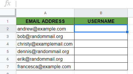
Say you have a list of email addresses. You want to extract the beginning of the email addresses, so only the username part until the ‘@’ character.

So how do we do that?

The SEARCH function is straightforward and easy to use. It only needs the text we search for and the text in which we search.

Let’s dive right into real examples to deal with actual values and see how to use the SEARCH function in Google Sheets.

The Anatomy of the SEARCH Function

So the syntax of the SEARCH function is as follows:

=SEARCH(search_for, text_to_search, [starting_at])

Let’s dissect this and understand what each of these terms means:

• = the equal sign is how we start every function in Google Sheets.
• SEARCH is our function. We will have to add the variables into it for it to work.
• search_for is a required field that represents the substring that we want to look for within the text.
• text_to_search is another required field that is the text to search for the first occurrence of search_for. It reads from left to right, so the first occurrence means the first from left.
• start is an optional field that represents the number to start the sequence. If you omit using it, the sequence will start at 1.
• starting_at is an optional field that represents the index within text_to_search at which we want to start the search. Its default value is 1, so it starts the search at the first character of the text.

In general, the SEARCH function needs to know what we are looking for (search_for) and in which text we are searching (text_to_search).

Optionally, we can also give a starting point at which to start the search (starting_at). This optional attribute might be useful mostly when you know that there are multiple occurrences of your search_for value, and you want to ignore the first (few) results.

As a result, the SEARCH function returns a number. This number represents the position of the first character of the first occurrence of the searched text.

⚠️ Now A Few Notes to Use SEARCH Function Even Better

1. It’s important to note that SEARCH is not case-sensitive, meaning that uppercase and lowercase letters do not matter. For example, “abc” will match “ABC“.
2. The FIND function is a very similar function to SEARCH. The FIND function also returns the position of a substring within a string. The only difference is that the FIND formula is case-sensitive while SEARCH is not. To compare text where uppercase and lowercase letters matter, use the FIND function.
3. Make sure that you don’t add your search_for and text_to_search attributes in reverse order. The arguments should be supplied in a different order than other text functions such as SPLIT and other well-known text functions.
4. The SEARCH function allows the use of wildcards. In search_for, you can use an ‘*‘ (asterisk) to match multiple characters or a ‘?‘ (question mark) to match any single character in text_to_search.
5. To find a literal ‘?‘ or ‘*‘ in the text, you should use a ‘~‘ character before the searched character, for example, ‘~*‘ and ‘~?‘.
6. The start argument can’t be greater than the length of text_to_search.
7. A #VALUE! error occurs when the given search_for is not found in the supplied text_to_search string.
8. Similarly, a #VALUE! error occurs when starting_at is less than zero or is greater than the length of the text_to_search string

A Real Example of Using SEARCH Function

The SEARCH function alone is rarely used since we don’t often need the numeric position of a text fraction. Rather we use it as part of other formulas.

For example, we can combine it with other text functions (for example, the LEFT function) and use it when finding a specific position for other functions.

Take a look at the examples below to see how we use the SEARCH function in Google Sheets.

In this example, we have a list of email addresses, and we want to extract the username (the left part) of these addresses.

We used the LEFT function to return a substring from the beginning of a string. Check out our article on how to use the LEFT function in Google Sheets to learn more about its use!

The LEFT function needs a position, and it returns the left part of a string until that specified position.

Since email addresses have a username, followed by a ‘@’ character, we used the SEARCH function to search for these ‘@’ characters in the cells. After that, we created the attributes of the LEFT function with the help of this result.

The function is as follows:

=LEFT(A2,SEARCH("@",A2)-1)

Here’s what this example does:

• We selected the cell where we wanted to show the result and started writing the LEFT function. We started writing it in cell B2.
• The LEFT function needs two attributes: the source text we want to use and the position where we want to cut it. The source text is obviously the email address we need to cut, so the cell A2.
• After that, the position where we want to cut the email address is calculated with the help of the SEARCH function. We started writing it as the second attribute.
• The SEARCH function first needs the search_for attribute, which is the ‘@’ character.
• Then, it needs the text_to_search attribute, which is the original email address, so we used the cell reference A2 here.
• The SEARCH function returns a number that is the position of the ‘@’ character.
• Finally, we need to subtract 1 from this position, because we don’t want to include the ‘@’ character in our result, only the part before.
• We applied the same function to the rest of the list by dragging it down through column B.
• As a result, we get the username parts of the email addresses until the ‘@’ character.

Simple, right?

You can give it a try yourself by making a copy of the spreadsheet using the link below:

How to Use SEARCH Function in Google Sheets

Let’s begin writing our own SEARCH function in Google Sheets step-by-step.

1. To start, click on any cell to make it the active cell. For this guide, I will be selecting B2.

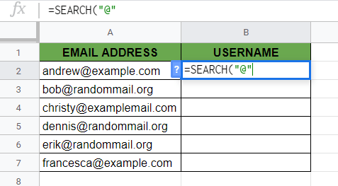
2. Next, type the equal sign ‘=’ to begin the function and then followed by the name of the function which is ‘search‘ (or ‘SEARCH‘, whichever works).

3. Great! Now you should find that the auto-suggest box will pop-up with the name of the functions starting with SEARCH. Select the right function (the one that is simply SEARCH) by clicking on it.

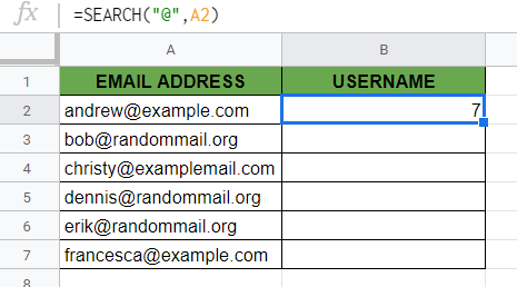
4. After the opening bracket ‘(‘, you have to add the attributes. Remember that you can add up to three attributes, and two of them are required, the third one is optional. In this example, we want to get the position of the ‘@‘ character, so we added it as the first attribute. Make sure to put this between “” double quotation marks since it is a direct textual value here.

5. After that, you need to add a comma and then the other required attribute which is the text_to_search. Here we want to search in the email addresses, so we reference the cell with the corresponding email address. So we will be selecting the cell B2 by clicking on it.

6. Hit the Enter key, and you can see the position of the ‘@‘ character in the email address! We got 7 here as a result, and indeed the seventh character is the ‘@‘.

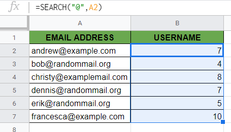
7. Drag down the function to the whole column to apply it for all the email addresses.

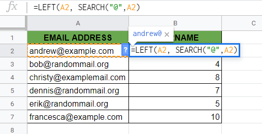
8. Now you might use this result as an index for other text functions. Let’s see our example with the LEFT function. Double click on the cell B2 to continue editing it.

9. After that, click between the ‘=’ equal sign and the SEARCH function and type the name of the LEFT function followed by the ‘(‘ opening bracket.

10. Now you should put the first attribute of the LEFT function here, which is the text you want to cut. Click on the cell that has your text. For example, here I click on the cell with the right email address, so on the cell A2. Put a comma next to this attribute, and you can already see the expected result.

11. Finally, there is only one more thing you need to do to extract the username. As you can see, the expected result includes the ‘@‘ character as well, which we don’t need. The position is defined by the result of the SEARCH function. Consequently, if you subtract 1 from the SEARCH formula (by writing -1 at the end of it), you will get the right result!

12. Hit on your Enter key to close the whole formula and get the result! Also, apply the modified function to the whole column. Now, if you followed our steps, you can see the extracted usernames.

That’s it, good job! You can now use the SEARCH function in combination with the other Google Sheets formulas to create even more powerful scripts that can make your life much easier. 🙂

Get emails from us about Google Sheets.

Our goal this year is to create lots of rich, bite-sized tutorials for Google Sheets users like you. If you liked this one, you'll love what we are working on! Readers receive ✨ early access ✨ to new content. There will be no spam and you can unsubscribe at any time.

Subscribe