


This guide will explain in detail how to show negative numbers as red in Excel.
Follow our guide to learn how to use conditional formatting and number formatting to display negative values as red text.
Excel’s conditional formatting feature is useful when you must change the formatting of a cell when certain criteria are met.
Let’s take a look at a quick use case where we can use conditional formatting to highlight negative numbers.
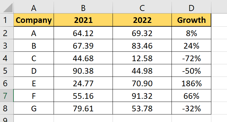
Suppose you are keeping track of several assets on the stock market. You have a spreadsheet that shows the growth of certain stocks from 2021 to 2022.
Growth is displayed as a percentage value that may be either positive or negative. You want to display negative numbers as red text to highlight how much of your portfolio has decreased in value over the past year.
Since we want to change the formatting of a number, we can use either conditional formatting or number formatting.
The main advantage of conditional formatting is that it has a more intuitive setup. The number of format codes you must use for the Format Cells feature are much harder to understand.
In this guide, we will explain how to show negative numbers as red using both methods.
Now that we have a grasp of when to format negative numbers, let’s explore a sample spreadsheet that uses both methods.
A Real Example of Displaying Negative Numbers as Red in Excel
The following section provides several examples of how to display negative numbers as red text. We will also go into detail about the formulas and tools used in these examples.
First, let’s take a look at our sample dataset. The dataset below computes the growth of certain stocks based on their average price in 2021 and 2022.
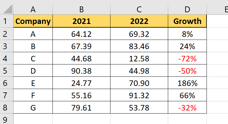
In the example below, stocks from companies C, D, and E have negative growth and appear in red. We’ve used conditional formatting to change how negative numbers appear in our sheet.
We can also use the built-in number format codes to achieve a similar effect.
In the Format Cells dialog, we can add the following custom formatting:
0.00%;[Red]-0.00%
Let’s take a closer look at what this custom format code is trying to do.
The format code is divided into two parts by a semicolon. When we specify two sections of format code, the first section of code will apply for positive numbers and zeros, and the second section of code is for negative numbers.
We must add the ‘[Red]’ format code in the second section to display negative numbers with red text. Excel only recognizes eight colors by name: Black, White, Red, Green, Blue, Yellow, Magenta, and Cyan.
Do you want to take a closer look at our examples? You can make your own copy of the spreadsheet above using the link attached below.
Use our sample spreadsheet to see if the colors of the growth percentage change when it is a negative number. Try changing the values of each stock to get a negative growth rate.
Want to try adding red formatting to negative numbers in your own sheet? Head over to the next section and read our step-by-step breakdown on how to do it!
How to Show Negative Numbers as Red in Excel
This section will guide you through each step needed to show negative numbers as red in Excel.
You’ll learn how we can use conditional formatting and number formatting to change how our number is displayed when it is a negative value.
Follow these steps to show negative numbers as red in Excel:
- First, let’s try using the conditional formatting tool to format our negative numbers.
Select the range that will require the formatting. In this example, we’ll choose cells D2:D8.

- Next, go to the Home tab and click on the Conditional Formatting option. Under the dropdown list, select New Rule.

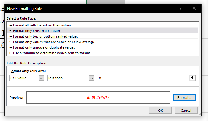
- In the New Formatting Rule dialog box, select the rule type ‘Format only cells that contain’. Next, set up the rule description to format only cells that have a cell value less than 0.

- Click on the Format option to determine. In the Format Cells dialog, navigate to the Font tab and select red as the font color. Click on OK to apply these formatting options.
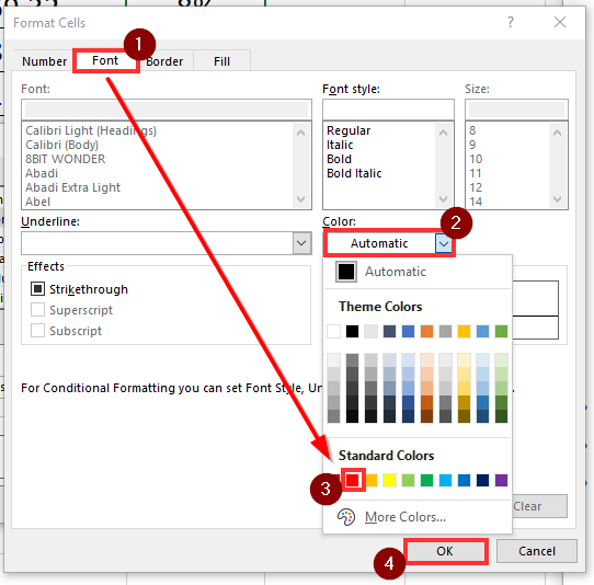
- The preview text should now show the proper formatting. Click on OK to apply the formatting rules to the selected sheet.
- In the example below, our negative values in the range D2:D8 are now formatted in red.
- Next, we’ll show you how to use custom number format codes to show negative numbers as red. First, select the range you want to format. In this example, we’ll use the range D2:D8 again.

- Type the keyboard shortcut Ctrl + 1 to access the Format Cells dialog pop-up. In the Number tab, you may choose to format negative numbers from a selection of default options.

- You may also add a custom number format code that works best with your data. For example, if you want to apply the red formatting to a percentage, you’ll have to add custom code similar to the string seen below.

These are all the steps needed to display negative numbers in your dataset as red text.
This step-by-step guide should provide you with all the information you need to display negative numbers as red text in Excel.
Conditional formatting is just one example of the many Excel features you can use in your spreadsheets. Our website offers hundreds of other functions and methods to help you get more out of Microsoft Excel.
With so many other Excel functions available, you can find one that is appropriate for your use case.
Don’t miss out on our team’s spreadsheet tips, tricks, and best practices. Subscribe to our newsletter to stay updated on the latest guides from us!


