SUBTOTAL Function in Google Sheets

This guide will explain how to use the SUBTOTAL function in Google Sheets.

The SUBTOTAL function in Google Sheets is a versatile function you can use to compute summary statistics like sum, average, count, max, and min on a range of cells. 

When working with a filtered dataset, the SUBTOTAL function can help summarize data while ignoring filtered rows as well as manually hidden cells. Each time the user adjusts the filter criteria, the SUBTOTAL function will automatically update to reflect the visible data.

In this guide, we will provide a step-by-step tutorial on how to use the SUBTOTAL function in Google Sheets.

The Anatomy of the SUBTOTAL Function

The syntax of the SUBTOTAL function is as follows:

=SUBTOTAL(function_code, range1, [range2, ...])

Let’s look at each argument to understand how to use the SUBTOTAL function.

• = the equal sign is how we start any function in Google Sheets.
• SUBTOTAL() refers to our SUBTOTAL function. This function accepts a vertical range of cells and an aggregation function and returns a subtotal using that function.
• function_code refers to the function to use to aggregate the subtotal.
  • AVERAGE (1)
  • COUNT (2)
  • COUNTA (3)
  • MAX (4)
  • MIN (5)
  • PRODUCT (6)
  • STDEV(7)
  • STDEVP (8)
  • SUM (9)
  • VAR (10)
  • VARP (11)
• range1 refers to the first range to calculate the subtotal of. You can add additional ranges (range2 and so on) after this argument to calculate more subtotals.
• Do note that you can include hidden values by increasing the number by 100. For example, a function code of 102 will run the COUNT function while skipping hidden cells.
• Using SUBTOTAL helps prevent double-counting associated with simple SUM formulas.

A Real Example of the SUBTOTAL Function in Google Sheets

Let’s explore a few examples of Google Sheets spreadsheets that use the SUBTOTAL function.

Using the SUBTOTAL Function On a Filtered Range

Let’s take a look at how we can use the SUBTOTAL function on a range of filtered data.

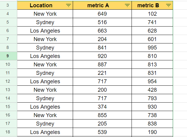
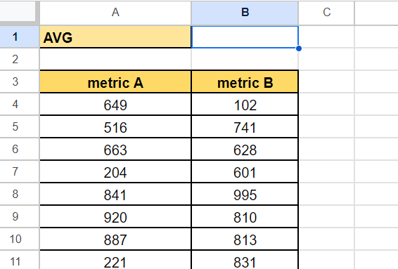
In the table above, we’ve added a filter that allows us to filter two different metrics by location.

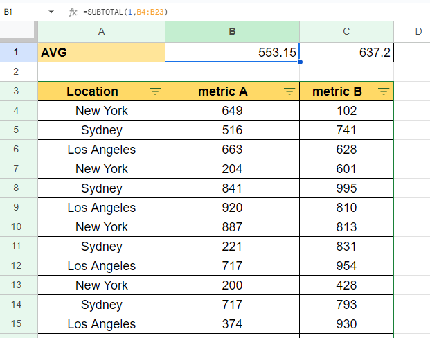
Suppose we want to summarize the average of each metric while also accounting for the current filter criteria. We can use the following SUBTOTAL formula to calculate this:

=SUBTOTAL(1,B4:B23)

The SUBTOTAL function allows us to aggregate data in different ways. Setting our function code to 1 will return the average of the specified range.

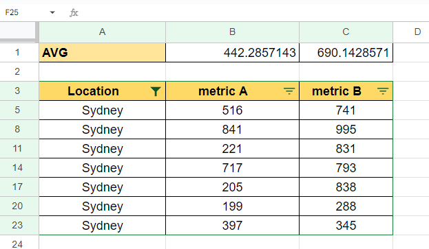
If we change the filter criteria to only show data points where the location is Sydney, our SUBTOTAL result will adjust accordingly.

Using the SUBTOTAL Function With a Dropdown List

Since the SUBTOTAL function can handle different types of aggregation functions, we can use the SUBTOTAL function repeatedly to summarize our data.

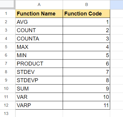
The table above will act as a lookup table for retrieving different function codes given a function name selected from a dropdown list. We’ll use the VLOOKUP function on this lookup table to provide the right function code for the SUBTOTAL function.

We’ll then use data validation on several cells to create dropdown lists listing each available function name.

Given that we want to summarize the range A2:A21, we can use the following formula to calculate the subtotal:

=SUBTOTAL(VLOOKUP(C1,'Function Codes'!$A$2:$B$12,2,FALSE),$A$2:$A$21)

The VLOOKUP function uses the function name and lookup table in the Function Codes sheet to return the appropriate function code. This code will change how our SUBTOTAL function summarizes our range.

Click on the link below to create your own copy of our examples.

Read the next section for a step-by-step tutorial on how to start using the SUBTOTAL function in Google Sheets.

How to Use the SUBTOTAL Function in Google Sheets

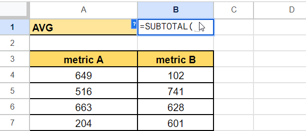
1. Click on the cell where you want the subtotal to appear.
   
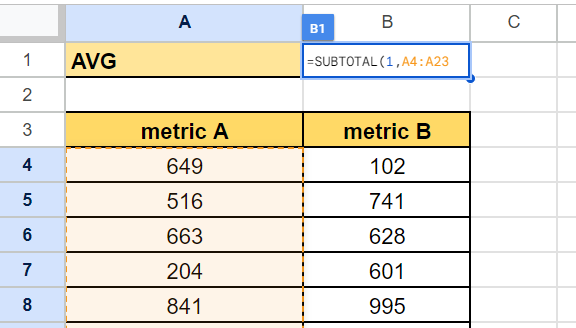
2. Type “=SUBTOTAL(“ into the cell to start the function.
   
3. Next, input the desired function number. This number determines what type of calculation the SUBTOTAL function will perform (e.g., 9 for sum, 1 for average, etc.).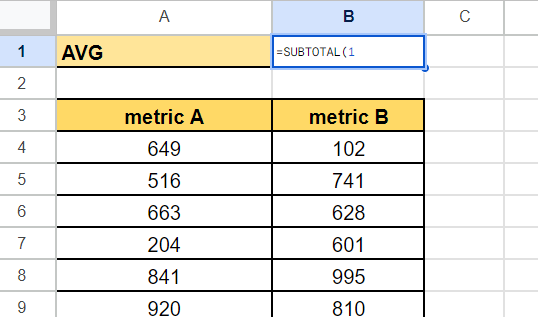
   In this example, let’s use 1 (AVERAGE) as the function number.
   
4. For the next argument, specify the range of cells you want to include in the subtotal.
   
5. Hit the Enter key to execute the SUBTOTAL function. The subtotal will be calculated and displayed in the selected cell.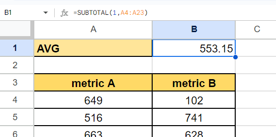
   In this example, we find out that the sum of our range is 11,063. 
   
6. We can include more ranges in our SUBTOTAL function by adding the range as another argument.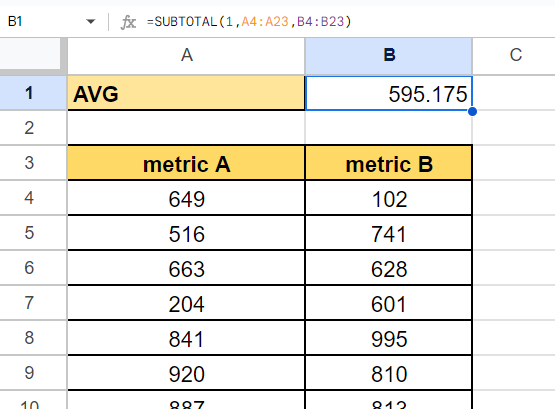
   
7. If you have filtered data, we recommend placing the SUBTOTAL function outside the filtered range.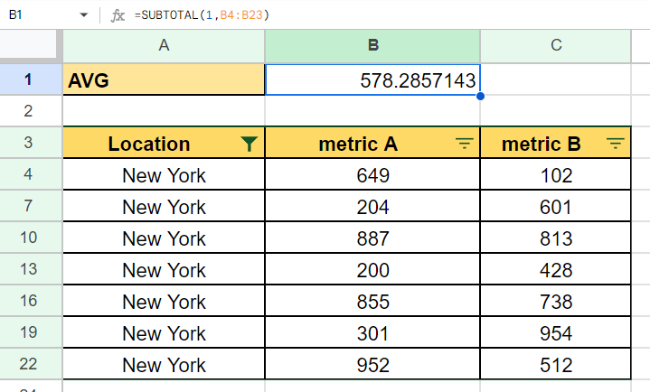
   SUBTOTAL will recalculate the aggregation after the user adjusts the filter criteria.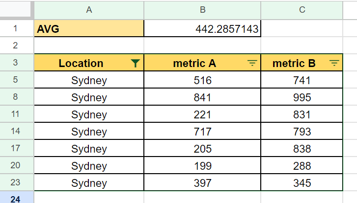
   

These are all the steps you need to know to start using the SUBTOTAL function in Google Sheets.

FAQs

1. What is the difference between the SUBTOTAL function and the typical aggregation functions like SUM, MIN, MAX, and AVERAGE?
   The SUBTOTAL function in Google Sheets offers more versatility compared to those functions. Since the aggregation function can be controlled by the first argument, users can create interactive dashboards that provide summaries using multiple SUBTOTAL functions. Additionally, SUBTOTAL can ignore values in rows hidden by filters, which these other functions are unable to do.
   
   
2. Is there a way to make the SUBTOTAL function in Google Sheets ignore hidden rows that were manually hidden, not by filters?
   When you add “10” to the usual function number (e.g., using 109 instead of 9 for SUM), the SUBTOTAL function will ignore all manually hidden cells that are part of the range.

To learn more about summarizing datasets in Google Sheets, you can read our post on how to use aggregation functions in Google Sheets.

That’s all for this guide! Be sure to check out our library of spreadsheet resources, tips, and tricks!