This guide will explain how to use the INDEX and MATCH functions to return a 2D array.
Table of Contents
INDEX and MATCH are powerful functions often paired together to create formulas capable of advanced lookups. The MATCH function finds the position of a lookup value in a range and the INDEX function uses that position to retrieve another value in the same row or column.
This level of flexibility makes it even more effective than functions like VLOOKUP function and HLOOKUP function which require the lookup value to be in a specific location. We can even modify our formula to output a 2D array instead of a single value.
For example, given a dataset with 12 columns, we can use INDEX and MATCH to return all columns up to a column header that matches some lookup value. If our column headers are the names of each month, we can use INDEX and MATCH to output all columns up to a certain target month.
In this guide, we will provide a step-by-step tutorial on how to use INDEX and MATCH to return a 2D array. We will look into how the formula works and later explore a working sample spreadsheet.
Let’s dive right in!
A Real Example of Using INDEX and MATCH for 2D Arrays
Let’s explore a simple example where we can use the INDEX and MATCH functions to return a 2D array.

In the table above, we have a sample dataset of monthly sales for five different products. We want to return a subset of this dataset starting from January up to April.

We can output our desired array by using the following formula:
=INDEX(A1:A6):INDEX(A1:G6,0,MATCH("April",A1:G1,0))
Let’s try to understand what each of the INDEX functions do. The formula INDEX(A1:A6) represents the first column to include in the desired array. The formula INDEX(A1:G6,0,MATCH(“April”,A1:G1,0)) uses INDEX and MATCH together to find the last column of our desired array.
The first argument of MATCH will determine what value to look for while the second argument refers to the range of cells to search through. We must set the third argument to 0 to only allow exact matches.
In our example, the MATCH function will return a value of 5 since ‘April’ appears in the fifth cell in the range A1:G1. This value will then be used as the third argument in the second INDEX to return the range E1:E6. The second argument will be set as 0 to allow the function to return the entire vertical range.
The addition of a colon (:) between both INDEX functions combines the output of the functions into multiple ranges. This allows the output to include all values between the first column and the last column of the source table.

In the table above, we modified the formula to work based on row headers rather than column headers.
In the second example, we want to return all rows until we reach Product B. We can output our desired rows as a 2D array through the following formula:
=INDEX(A1:G1):INDEX(A1:G6,MATCH("B",A1:A6,0),0)
Instead of using A1:A6 to refer to our starting column, we’ll use the range A1:G1 to refer to our starting row. We’ll also need to move our MATCH function to the second argument of its INDEX function since the second argument handles columns. We’ll set the third argument to 0 to allow the function to return the entire horizontal range.
Click on the link below to create your own copy of our examples. Use these examples to see how our INDEX-MATCH formulas work.
Head over to the next section to follow our step-by-step guide on how to get started using INDEX and MATCH to output a 2D array!
How to Use Index with Match for 2D Array Result in Google Sheets
- First, use the
INDEXfunction to output the first column to include in our 2D array output.

- Next, add a colon character after the first
INDEXfunction. The colon indicates we want our formula to return a matrix (2D array) output.

- After the colon, start writing the
INDEX-MATCHformula that will try to match a column with the appropriate column header. In the formula below, we want to return the column with “April” as its column header.

- Hit the Enter key to evaluate the function. The output of the function should include the target range up to the matched column.

- We can modify our formula to match row headers instead. Instead of specifying a starting column and a target column, we’ll convert the formula to reference rows in the target range instead.

That’s everything you need to know to start using INDEX and MATCH together to return a 2D array in Google Sheets.
FAQs
- What is the purpose of the colon in the INDEX-MATCH formula?
The colon character is primarily used to identify ranges. The colon appears between two cell references of a range to denote that the range includes all cells between the first and last cells.
In ourINDEX-MATCHformula, the colon between twoINDEXfunctions allows us to create multiple ranges for each pair of values from theINDEXfunctions.
- Can I use an arbitrary starting point when using INDEX and MATCH for returning a 2D array?
Yes, it is possible to set up an arbitrary starting row or column. We simply need to use anINDEX-MATCH,formula for both the starting and ending rows or columns.In the table above, we usedINDEXandMATCHto find the row with a ‘B’ value and a row with a ‘D’ value. A colon is placed between these two formulas to create a 2D array.
INDEX and MATCH are just two of many built-in functions available in Google Sheets. Another way we can extract data from a range is through the CHOOSEROWS function and CHOOSECOLS function.
If you want to learn more advanced spreadsheet techniques like this, try browsing our library of Google Sheets resources, tips, and tricks!