This guide will explain how to use SUMPRODUCT across multiple sheets in Excel.
The rules for using the SUMPRODUCT function in Excel are the following:
- The
SUMPRODUCTfunction will multiply the range or array together and return the sum of the products. Additionally, the function can support up to 30 ranges or arrays. - The function will treat non-numeric values in the data set as zeros.
- So the inputted array or range arguments must have the same size or dimensions. Otherwise, the function will return a #VALUE! error.
- When we have logical tests inside the arrays or ranges which will create TRUE and FALSE values, we would want to convert these values to 1s and 0s.
Excel is an excellent tool to use when performing difficult and long calculations. When we deal with large amounts of data, we can easily organize and manipulate them in Excel. Since there are several built-in functions and tools in Excel, we can utilize them for different purposes and situations.
In this guide, we will focus on learning how to use the SUMPRODUCT function across multiple sheets. So the SUMPRODUCT function is used to get the sum of the products of the selected range or array. Basically, it will first multiply the values in the range or array. Then, it will sum all the products together.
To use this function across multiple sheets, we will combine it with the SUMIF and INDIRECT functions. So we can create a formula using these three functions to get the sum of the products across multiple sheets.
Let’s take a sample scenario wherein we must use SUMPRODUCT across multiple sheets in Excel.
Suppose we have a data set containing the number of sales for different products. Furthermore, we have created multiple monthly data sets and placed them in multiple sheets. So we created a formula using the SUMPRODUCT, INDIRECT, and SUMIF functions to get the desired result.
Before we move on to a real example of using SUMPRODUCT across multiple sheets in Excel, let’s first learn how to write the different functions we will be using.
The Anatomy of the SUMPRODUCT Function
The syntax or the way we write the SUMPRODUCT function is as follows:
=SUMPRODUCT(array1, [array2])
Let’s take apart this formula and understand what each term means:
- = the equal sign is how we begin any function in Excel.
- SUMPRODUCT() refers to our
SUMPRODUCTfunction. And this function is used to return the sum of the products of corresponding ranges or arrays. - array1 is a required argument. So this refers to 2 to 255 arrays which we want to multiply and then sum the values. Additionally, all the selected arrays must have the same size or dimensions.
- array2 is an optional argument. And this serves as a supplement to the first argument. So this also refers to 2 to 255 arrays which we want to multiply and then sum the values.
The Anatomy of the INDIRECT Function
The syntax or the way we write the INDIRECT function is as follows:
=INDIRECT(ref_text, [a1])
Let’s take apart this formula and understand what each term means:
- = the equal sign is how we start any function in Excel.
- INDIRECT() is our
INDIRECTfunction. And this function is used to return the reference specified by a text string. - ref_text is a required argument. So this refers to a cell reference containing an A1- or R1C1-style reference, a name defined as a reference, or a cell reference as a text string.
- a1 is an optional argument. And this refers to a logical value that will specify the type of reference the ref_text argument is using. When we input FALSE, we refer to an R1C1 style. Otherwise, TRUE or omitted, we refer to an A1-style.
Great! Now we can move on and dive into a real example of using SUMPRODUCT across multiple sheets in Excel.
A Real Example of Using SUMPRODUCT Across Multiple Sheets in Excel
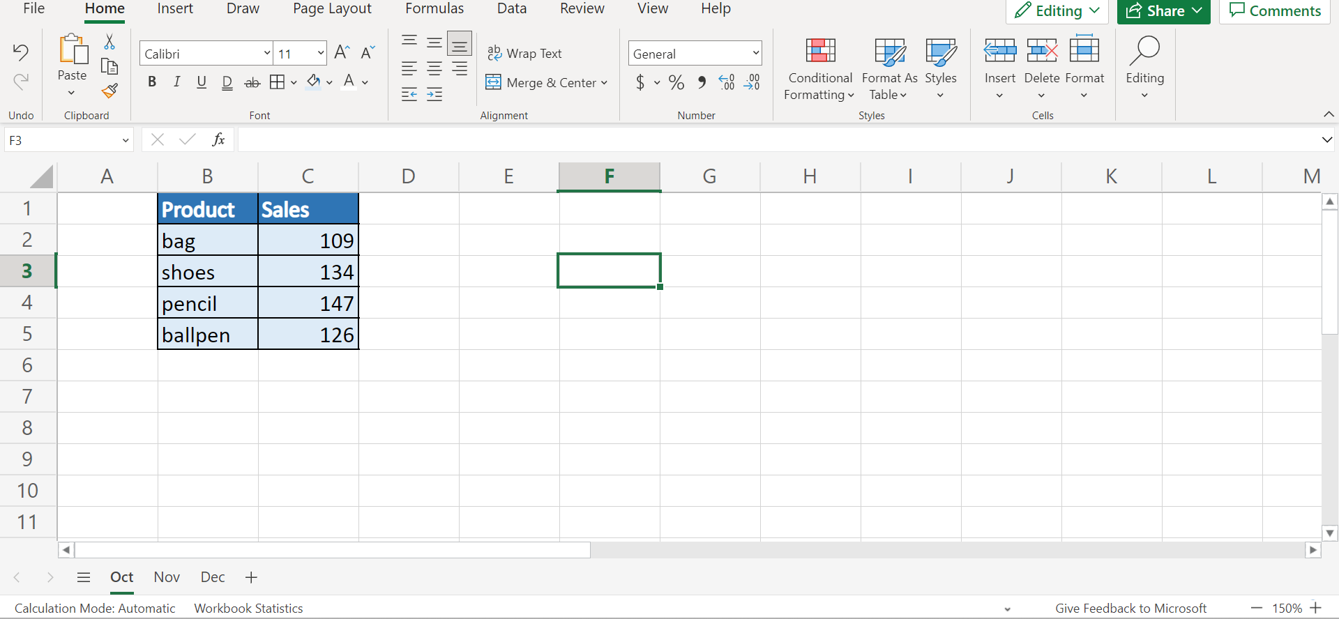
Let’s say we have a data set containing the number of sales for each product. And we separated the sales for each month into different sheets. Thus, we have three separate sheets for the sales for the month of October, November, and December. So our initial data set would look like this:
In this example, our goal is to use the SUMPRODUCT function to get the total number of sales for the three months, which is found across multiple sheets. Luckily, we can combine the SUMPRODUCT function with the INDIRECT and SUMIF functions to perform this task.
So the INDIRECT function is used to return a reference specified by a text string. In Excel, references are immediately evaluated to display their contents. Usually, we use this function when we want to change the reference to a cell within a formula without changing the formula itself.
Then, the SUMIF function is used to add cells specified by the condition or criteria we set. To use this formula, we first need to create a new sheet that will act as the summary to display the result. Then, we will make the same table found in the other sheets containing the product and total sales.
Next, we will create a table containing the names of the different sheets. Afterward, we can input the formula in the first cell of the data set in the summary sheet. Then, we can drag down to copy the formula and get the result for the other cells.
Additionally, we must use the absolute reference in our formula so that the reference does not change as we drag down the formula. In this case, the sheet names were used in the formula. Next, the product names were used as the product names of the reference sheets.
So our final data set would look like this:

You can make your own copy of the spreadsheet above using the link attached below.
Amazing! Now we can proceed and explain the process of how to use SUMPRODUCT across multiple sheets in Excel.
How to Use SUMPRODUCT Across Multiple Sheets in Excel
In this section, we will explain the step-by-step process of how to use SUMPRODUCT across multiple sheets in Excel. Furthermore, each step has detailed instructions and pictures to guide you along the process.
1. Firstly, we will create a new sheet. To do this, we will look to the bottom and click the “+” sign beside the sheets.

2. Secondly, we will right-click the sheet and select Rename.

3. Thirdly, we will type in “Summary” and click OK.

4. Next, we will create the same table found in the other sheets containing the same product names and an empty column for the total sales. Additionally, we will make a column containing the names of the sheets.

5. Afterward, we can now use the formula. So we will type in the formula “=SUMPRODUCT(SUMIF(INDIRECT(“‘”&$B$8:$B$10&”‘!$B$2:$B$5”),B2, INDIRECT(“‘”&$B$8:$B$10&”‘!$C$2:$C$5”)))”. Lastly, we will press the Enter key to return the result.

6. Then, we will pull down the Fill Handle tool to copy the formula and apply it to the other cells.

7. And tada! We have successfully used SUMPRODUCT across multiple sheets in Excel.
And that’s pretty much it! We have explained thoroughly how to use SUMPRODUCT across multiple sheets in Excel. Now you can apply this method to your work whenever you need to.
Are you interested in learning more about what Excel can do? You can now use the INDIRECT function and the various other Microsoft Excel formulas available to create great worksheets that work for you. Make sure to subscribe to our newsletter to be the first to know about the latest guides and tutorials from us.