You can use the CORREL function to calculate the correlation coefficient of two variables in Google Sheets.
In statistics, one way to determine how closely related two sets of data are is to find their Pearson correlation coefficient known as Pearson’s r. The formula for finding Pearson’s r is quite complex, but with Google Sheets, you don’t need to worry.
You can easily calculate the correlation coefficient of two datasets using a simple function called CORREL. Learn more about this function by reading through this article.
What is Pearson Correlation Coefficient?
The Pearson’s r is a statistical metric used to calculate the linear association between two variables. This metric returns a value between -1 and +1, with +1 implying a perfect linear relationship and -1 as a perfect negative relationship. If Pearson’s r of two variables is 0, then these variables don’t correlate.
For you to better understand Pearson’s r, take a look at the graphs below.
Negative Correlation
Two variables have a negative correlation when their correlation coefficient is negative. As the x increases, the y decreases.

Looking at the Scatter chart above, it is possible to draw a trendline across the data points. We can then infer that there is a significant relationship between the variables. If the correlation coefficient is exactly -1, it’s a perfect negative correlation.
Positive Correlation
When two variables have a positive correlation, more specifically, the closer their correlation coefficient is to 1, the more significant relationship they have.

In the chart above, you can still easily draw a trendline connecting the data points. This means that the variables have a linear relationship. In cases wherein the correlation coefficient of two variables is exactly +1, expect that data points would be in a perfect straight line.
No Correlation
If the resulting correlation coefficient of two variables is equal to, or close to 0, the data points would appear scattered along the chart. This signifies that there’s no significant relationship between the variables.

Notice that, in the above chart, you cannot even trace a meaningful trendline across the data points.
Using the CORREL Function to Calculate a Correlation
Calculating the correlation of two variables in Google Sheets is very easy, thanks to the CORREL function. Of course, to use it, you must first understand its syntax.
Here’s how you should write the CORREL function in Google Sheets:
- = the equal sign is the first character we need to type in to initiate the
CORRELfunction in Google Sheets. - CORREL() this is our
CORRELfunction. - data_y is the parameter that will hold the cell range or array containing the values of the dependent data.
- data_x is the second required parameter, which will hold the cell range or array of the independent data.
The syntax of the CORREL function is fairly straightforward as you can see. You only need to supply two required parameters for it to work.
A Real Example of Calculating a Correlation in Google Sheets
This time, let’s have a look at how the CORREL function is implemented in Google Sheets.
Here is a spreadsheet that contains a set of variables.

To determine the extent of correlation between these variables, we can simply use the CORREL function, specifying the y column as the data_y parameter, and x column as the data_x parameter. Once implemented, the CORREL function will return this result:

The CORREL function in our example returned a positive value. It means that the variables have a positive correlation. When the result is plotted in a Scatter chart, you’ll have an output like this:

If you would like to have a copy of our example, go ahead and click the link below:
How to Calculate Correlation in Google Sheets
At this point, let’s learn the step-by-step process of using the CORREL function to calculate a correlation coefficient in Google Sheets.
- To start with, open the spreadsheet that contains the variables you wish to find the correlation coefficient for. Feel free to grab a copy of our example spreadsheet earlier if you just want to practice first.
- With the spreadsheet already open, click the cell where you want to display the result of the
CORRELfunction. In the example below, cell C2 is selected.

- Next, initiate the
CORRELfunction by typing in ‘=CORREL()’.

- Inside the parentheses of the
CORRELfunction, we can now specify the required parameters. For the first parameter (data_y), type in the cell range containing the dependent data.

- Right after the data_y parameter is where you’ll need to specify the data_x parameter. Here, type in the cell range containing the independent data.

- Once the parameters have been specified, press the Enter key on your keyboard. This should return the correlation coefficient of the variables in your spreadsheet.

- Great job! Now you know how to calculate the correlation coefficient of two variables in Google Sheets. If you want to visualize the correlation or trend of the variables, you can use the scatter plot feature of Google Sheets in your spreadsheet. Using this feature in our example dataset will give us this result:

There you have it! That’s all there is about using the CORREL function to calculate a correlation coefficient. You can use this function along with other functions in Google Sheets to illustrate your data clearly and more effectively.
Interested in learning more about Google Sheets functions? Then check out our other articles in Google Sheets.
Subscribe to our newsletter to keep up with the latest about Google Sheets.