While there are no built-in functions in Google sheets to count cells based on the cell color, you can achieve the same result using a custom function written in the script editor. Read through the guide to understand how to write one.
You don’t need to write the function yourself, should that not be your cup of tea. There are plug-ins you can use for this utility – like PowerTools or Function by Colour. They have a month-long trial version with an option for a subscription – for 12 months or a lifetime. Both of them are outside of this guide’s scope.
Let’s take an example.
I have marks secured by students in each batch of my private tuition classes in last week’s takeaway test, formatted using conditional formatting – highlighted in green color for marks greater than 75 and highlighted in red color otherwise. I could very well filter the marks column and get the count of students who passed (for every batch), but it would be a time-consuming job.
And this is where counting cells based on their color can help me save time.
Real Example of Counting Cells Based on Cell Color
Take a look at the example below to see how you can count cells based on cell color in Google Sheets:

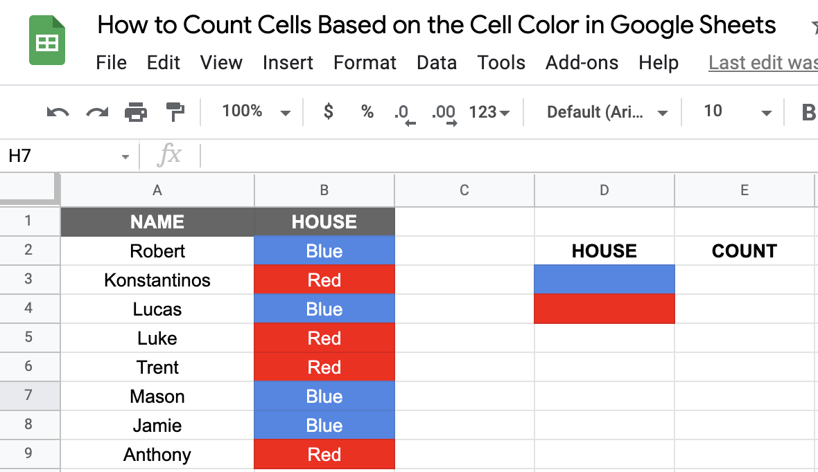
The given above are a group of students and their respective houses (or groups) that they have been divided into at school. The objective here is to find the number of students allotted to each house (red and blue) based on the cell color.
As you can see below, I have obtained the desired result using a custom function:

You may try changing the colors and see how the result changes. Go ahead and make a copy of the spreadsheet using the link I have attached below:
So, how do you write your own custom function in Google Sheets? Let us take a detailed look at it with the help of an example.
How to Count Cells Based on Cell Color in Google Sheets
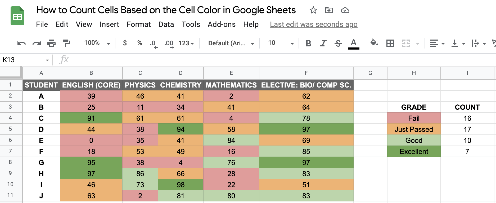
- I have listed the marks secured by high school students in the neighborhood school in their annual examinations, by subjects. If you notice carefully, I have color-coded their performance into four categories – ‘Failed’ (red), ‘Just Passed’ (orange), ‘Good’ (light green), and ‘Excellent’ (dark green). The objective is to find out the distribution of students across the four categories, across all the subjects.

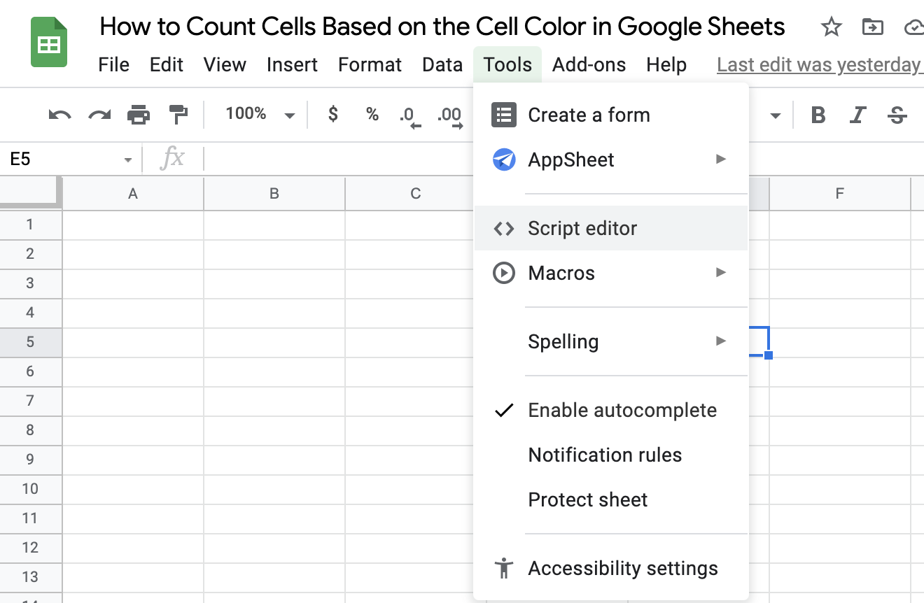
There is a provision called Script Editor in Google Sheets. Navigate to Tools → Script Editor

Clicking on the ‘Script Editor’ should redirect you to a new window that will allow you to write your code, as shown below.

- Once you are here, go ahead and write the script that gets you the desired function capability – in this case, counting the cells based on their color. Once finished, hit the save button, and the function will now be available in your Google Sheets for further use.

Custom Function particulars
Let me try to explain the logic line-by-line.
-
- Line 1: denotes the name given to the function and the inputs required by it to execute it. The given name, in this case, is ‘countColoredCells’, which requires two-parameter inputs – countRange and colorRef.
- Line 2: the .getActiveRange() command will return the range selected by the user.
- Line 3: the .getSheet() command will return the active sheet.
- Line 4: the .getFormula() returns the formula applied to the top-left cell of the selected range.
- Lines 6-9: denote selecting the range and the background color, respectively. The .getBackgrounds() returns the value for the background color.
- Lines 11-13: denote obtaining the reference background color to be matched.
- Line 15: initializes the count. This variable will update within the loop for every instance where the reference color matches the cell color.
- Lines 17-21: denote the loop that calculates the count for each reference color specified.
3. Come back to the Google Sheet and simply click on any cell to make it the active cell. For this guide, I will be selecting I4, where I want to show my results.
4. Next, simply type the equal sign ‘=‘ to begin the function and follow the function’s name, which you have named in the Script Editor. For this example, the function’s name is countColoredCells.
- As per the logic I have coded, two inputs are required – the range and the color reference. Enter both the inputs to the function and close the brackets, as shown below:

- Finally, just hit your Enter key. You will notice that the number of students in each of the groups has been counted against the respective color, making for easy reading of the summarized result. The sum of these counts is 50, which is equal to the total number of student-subject combinations, so the function has given the correct result as desired.

That’s pretty much it. You have everything you need to get started with counting cells based on the cell color. You can additionally try to sum the values based on color too. I recommend experimenting with the custom function, combining it with the numerous Google Sheets formulas available, and seeing what you can come up with. 🙂


