The MIRR function in Google Sheets is used to calculate the modified internal rate of return on an investment based on a series of periodic cash flows and the difference between the interest rate paid on financing versus the return received on reinvested income.
Table of Contents
The MIRR function is used to find the modified internal rate of return. The modified internal rate of return is a term in finance that refers to a scenario where the positive cash flows are reinvested using the firm’s cost of capital, with the initial payments financed at the firm’s financing costs.
The MIRR is useful because it creates a single solution, instead of comparing different cases of IRRs. Because some cases that you might need compare are vastly different, the MIRR brings that to a calculation that helps you see the projects from the same view.
The MIRR different from the internal rate of return as IRR assumes that the positive cash flows are reinvested using the IRR instead. Because of this, the MIRR can be considered a more accurate or realistic representation of the project.
The IRR is a simplified method that can sometimes result in an overstated percentage. This can affect decisions that are being made and hurt the capital budgeting procedure. The MIRR improves this by adding another assumption into the equation.
Let’s look an at example.
You want to choose what equipment to buy for your business. You have the information about each equipment’s useful life, how much profit it will add to your business, and how much it can be sold at the end of its useful life.
How should we go about this problem?
The MIRR function needs you to set up a table of cash flows, as well as know your financing rates and reinvestment return rates in order to study each equipment and make a sound financial decision.
The Anatomy of the MIRR Function in Google Sheets
The syntax of the MIRR function is as follows::
=MIRR(cashflow_amounts, financing_rate, reinvestment_return_rate)
Let’s have a look at each part of the function to understand what is going on here:
=is the equals sign that starts off any function in Google Sheets.MIRRis the name of our function.cashflow_amountsis the input of the function. Choose an array or range containing the income or payments associated with the investment. Note that it should include at least one negative and one positive cash flow to calculate the rate of return.financing_ratesis the interest rate paid on the funds invested.reinvestment_return_rateis the return (a percentage) earned on the reinvestment of income received from the investment.
You should also note that the perspective you are solving the problem from also matters.
If you are the owner of the investment, the cashflow_amounts will represent income, so they should be positive.
If you are the perspective of someone making a loan repayment, the cashflow_amounts will represent payments, so they should be negative.
A Real Example of Using the MIRR Function
Let’s look at the example below to see how to use MIRR function in Google Sheets.
Calculating the Modified Internal Rate of Return in Google Sheets
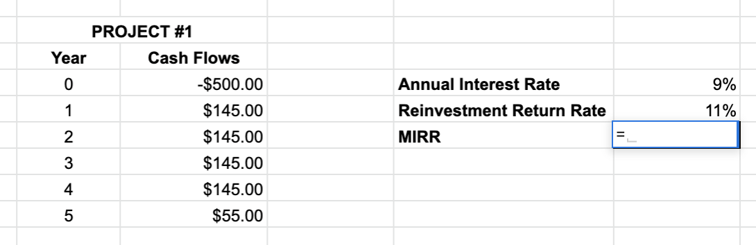
This is a simple problem. We want to find the modified internal rate of return for a certain project. Here in the example, the cash flow is laid out, as well as the interest rate paid on the funds invested and the reinvestment return rate.

The function takes three arguments. So in the equation, it will look like:
=MIRR(C4:C9,F4,F5)
As a result, we get 11.90%.
To further the point, let’s also get the IRR of the same project:

=IRR(C4:C9)
As a result, we get 12.81%.
You’ll notice that the IRR is indeed overstated, and thus the MIRR is a more conservative way to evaluate projects and profitability.
This simple problem can be practiced to perfection. Use the link below to get a copy of this problem set:
How to Use the MIRR Function in Google Sheets
In this section, we will show you a step-by-step process on how to use the MIRR function in Google Sheets.
In this problem, we will be comparing three different projects. The information that you have is laid out over three different cases. They are all projects that are not easy to compare at first glance, because they have different costs and different cash flows to offer the company.
You know that MIRR is usually used to compare projects of different scales and sizes.
It’s up to you, as project manager, to decide which project will benefit the company the most. You have decided to use the MIRR to compare these projects, and evaluate them after you have calculated for their MIRRs.
Calculating and Comparing MIRR in Google Sheets
- To begin, click on a cell to make active, which you would like to display the MIRR. For the guide. The MIRR will be in Cell F6.

- Next, type the equal sign ‘=’ to start writing the function. Follow this with “MIRR” or “mirr” – Google Sheets functions are not case sensitive so either is fine.
- The auto-suggest box will create a drop-down menu. Select the
MIRRfunction by clicking it. It is the first to pop up on the list, but take care to choose the correct function.

- After the opening bracket ‘(‘, you will add the range attribute. Drag your cursor over the entire cash flow column.

- Next, choose the financing rate.
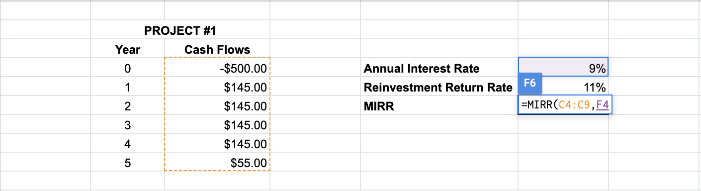
- Next, choose the reinvestment return rate.

- You will notice that there will be a preview of the result when you complete the inputs. Hit enter! You can now see the MIRR of the project you are working on.

- Do the rest of the sets – and make your decision as project manager!

Given a practical problem where you should completely solve for the return on investment, use MIRR to find and compare the rates of return of the other projects.
And there you have it – you can now use the MIRR function in Google Sheets together with the other numerous Google Sheets formulas to create even more effective formulas.