


Learning how to create a dependent drop-down list in Google Sheets is useful to create several lists of options for users to select from.
It is no surprise that most of us are well versed in creating dropdowns using the data validation feature in Google Sheets.
If you are not familiar with the data validation feature, do not be shy to check out our tutorial on how to use it, and learn through real-life examples for better understanding! 😇
Table of Contents
Let’s take an example:
Imagine you are a supplier for chairs. Your main income derives from selling office chairs and restaurant seatings.
Your catalog contains hundred types of chairs from many different brands. It is always a hassle when taking orders from companies in bulk as there would be errors in the data collected.
By using the dependent drop-down list in Google Sheets, we are able to minimize the errors and collect cleaner and more reliable data.
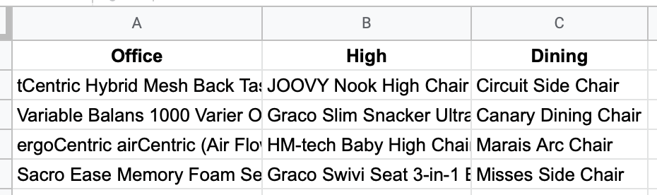
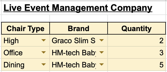
As shown above, using the dependent drop-down list we are able to let the users select which type of chairs and what brands to order.
Let us use a real-life example as a guide to learn how to create a multi-row-dependent drop-down list in Google Sheets.
You may make a copy of the spreadsheet using the link I have attached below.
A Real Example of Using Dependent Drop Down List Feature
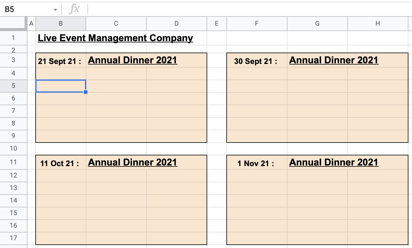
In this example, you are an Italian catering company that supplies food for different events.

For customers like event management companies, they have several events lined up that would need you to cater to. This makes it easy to make errors in the order form collected from your customers.
Let us create a multi-row dependent dropdown list in Google Sheets containing all the dishes from the menu for customers to select from.
This enables the customers to dependently select the dishes according to the events and the number of courses they want in an event.

Once the dependent dropdown list is created, we will be able to send this list through email to customers for them to list down all the dishes they want for each event.
How to Use the Dependent Drop Down List Feature in Google Sheets
Creating a multi-row dependent dropdown list in Google Sheets requires:
- First Dropdown List
- Prep Data List
- Second Dependent Dropdown List
The tedious part that needs more attention is when we are preparing the Prep Data List. It requires us to utilize several functions in a single formula.
Before you start, it is preferred to create three different sheet tabs for the Dependent Dropdown List, Master List, and Prep Data List.
![]()
This will enable your Google Sheets to be cleaner and easily navigated.
Second, you will also need to name the different ranges of data. This enables formulas to be easily understood and read.
For example, data within the cells of B5:B9 are named as Appetizers.

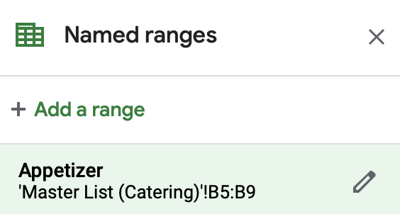
To do this, select Data, then Named ranges.

In the pop-up, input the desired name for the range of cells and select the range of cells to be named.

Take note that names inputted can only be a single word. If you want to put multiple words, input an underscore in between the words instead of pressing the spacebar.
Remember to categorize the remaining courses as well!
(a) First Dropdown List
- Let us create the first dropdown list. Simply click on the cell that you want to create your dropdown at. In this example, it will be B5.
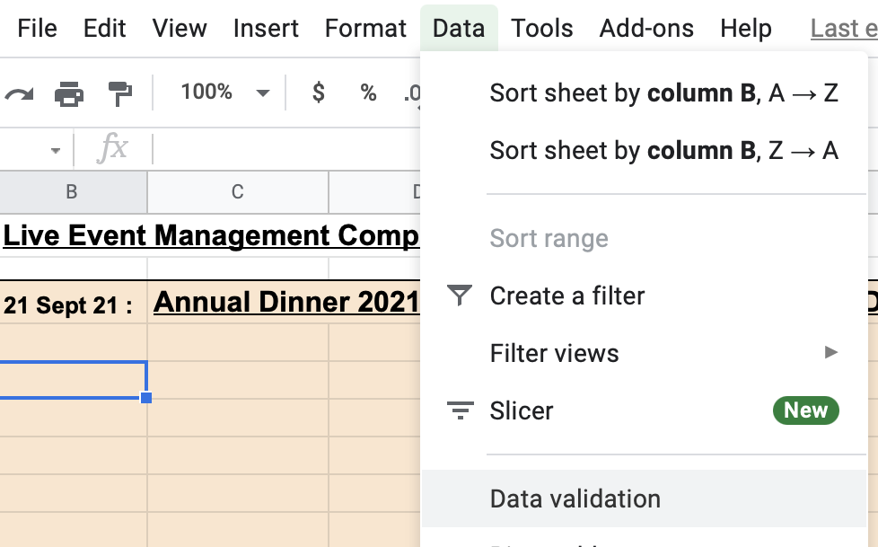
- Then, we will need to use the data validation feature to create a dropdown list. Press Data, then Data validation.
- In the pop-up box, we will select List from a range in the Criteria section and define the range as ‘Master List (Catering)’!B4:F4. This will enable us to create a dropdown list showing the five different courses for customers to select from.
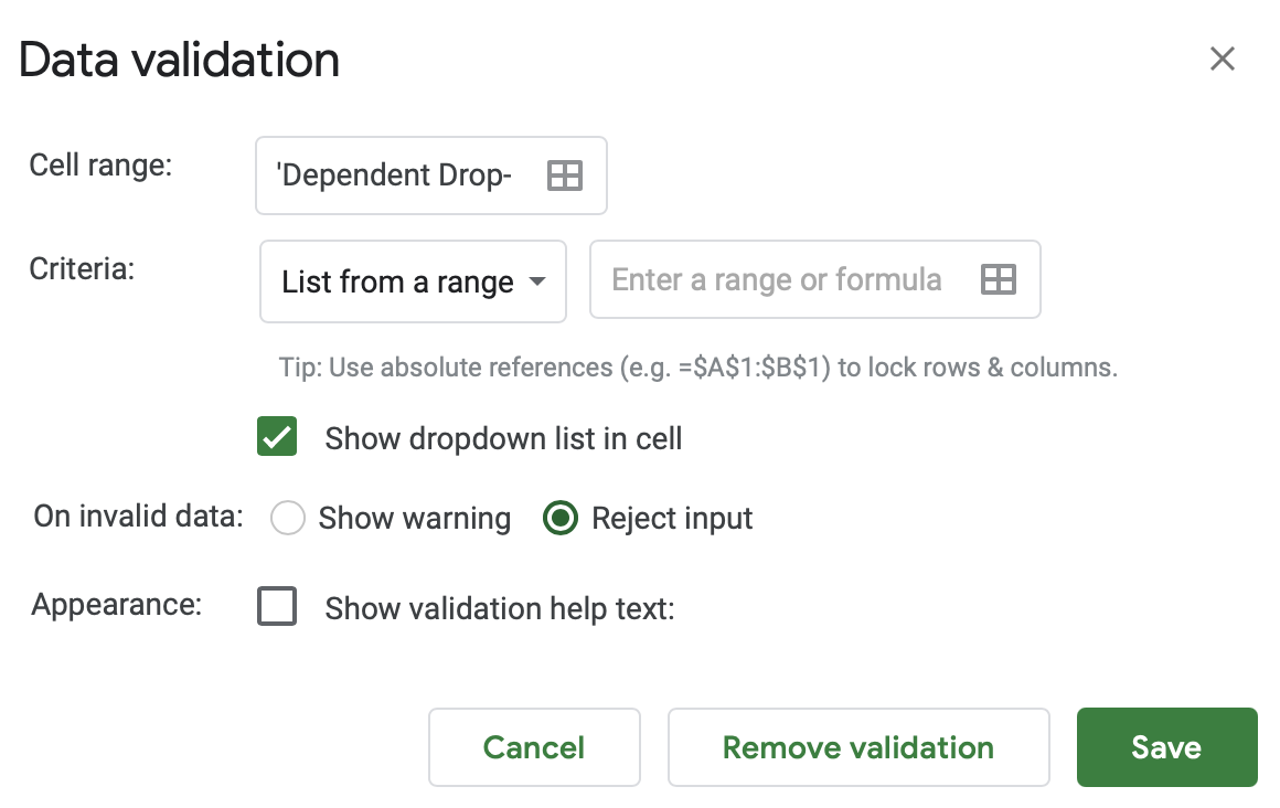

- Be sure to tick Show dropdown list in cell and select Reject input. You can also create a validation help text if desired.
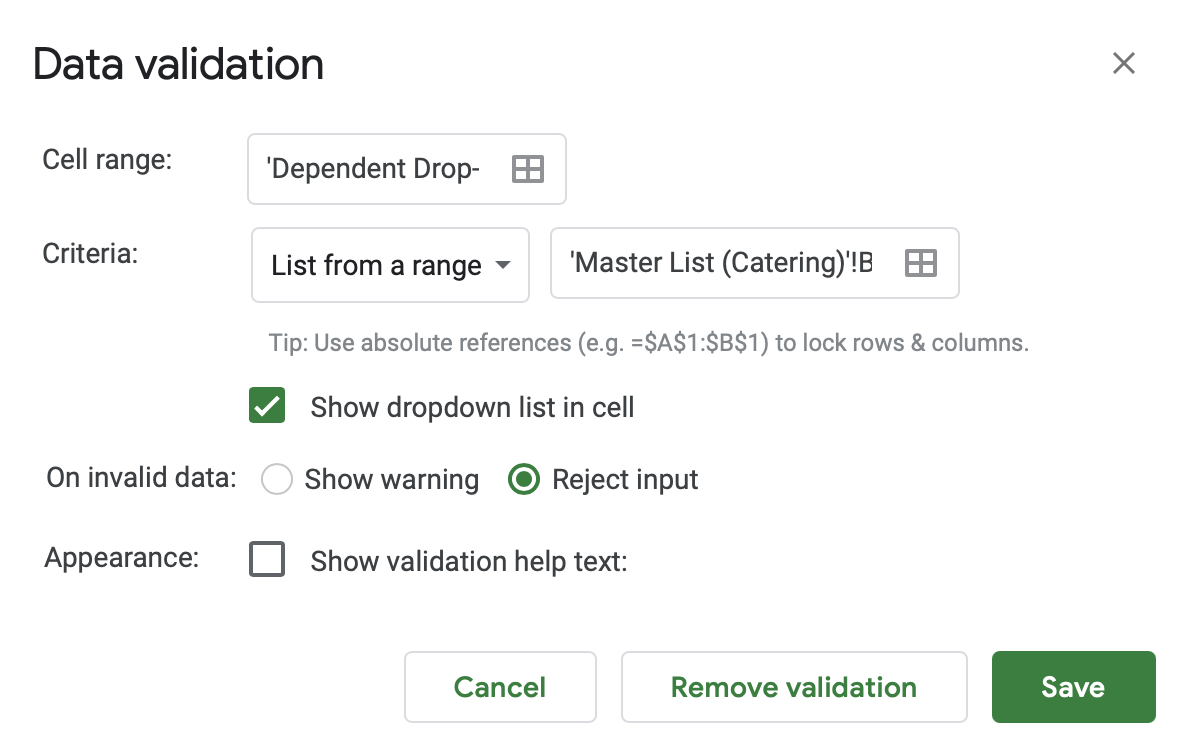
- Once you press Save, a dropdown list is created with the five different courses from your Master Listing.

(b) Prep Data List
The reason for preparing a separate data list is because the data validation feature does not allow us to enter formulas directly.
As the Second Dependent Dropdown List is reactive to the First Dropdown List, we will prepare a separate data list using several functions in Google Sheets to help us link them together.
Follow the steps slowly, and I will explain why we use each function for your better understanding at the end.
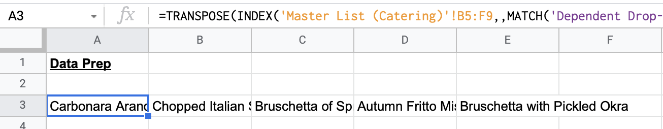
- First, create a separate sheet tab for the Prep Data List. Click on the cell you want to write your function in. In this example, it will be A3.

- Then, input this formula into the cell.
=TRANSPOSE(INDEX('Master List (Catering)'!B5:F9,,MATCH('Dependent Drop-down (Catering)'!B5,'Master List (Catering)'!B4:F4,0)))
- Once you press Enter, the list of appetizers will appear.
Let me explain how this formula works. Here is a visual representation of the entire formula:

First, the TRANSPOSE function is to help swap an array of data from columns to rows.
Second, the INDEX and MATCH functions help us to look up data from the Dependent Drop Down tab to the Master List.
The first argument in the INDEX function is to locate all the data located in cell B5:B9 in the Master List.

The second argument in the INDEX function is to specify which rows to return. Since we wanted all the rows to return, we left it blank.

In the third argument, we used the MATCH function to match the course selected in the Dependent Drop-Down tab to the range of courses in the Master List tab. We input ‘0’ as the match_type as we want the exact match to return.
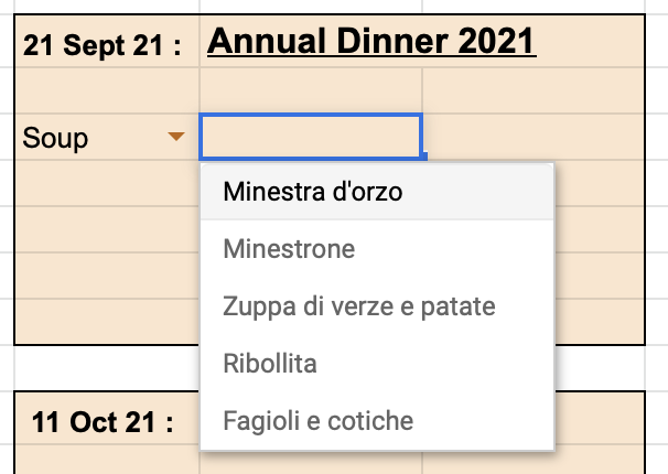
Hence, if in the Dependent Drop-Down tab we select Soup for the dropdown in B5, the formula in the Data Prep Tab will return the list of dishes for Soup.
(c) Second Dependent Dropdown List
Finally, we can create a data validation for creating the dependent dropdown list.
- First, select the cell you want to create the dependent dropdown list in. In this case, it is C5.
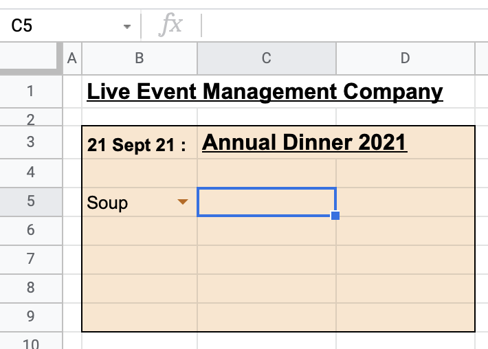
- Similar to the steps above, press Data, Data validation. Select List from a range as the criteria. For the range of cells, input the cells in Prep Data tab, ‘Data Prep (Catering)’!A3:E3.

- Once you press Save, a dropdown is created. The dropdown list will vary depending on the courses you choose in column B.
Once you fill in the formulas for all the other cells, your sheet will look something like this.
There you go! You have successfully created a dependent dropdown list!
If you are still unclear with any of the functions used within this tutorial, you can also check out our tutorials on how to use the TRANSPOSE, INDEX and MATCH functions for a better understanding!


1 comment
This works fine for a single cell but if you want to apply this validation to an entire sheet of entries, based on the method you use above either every entry will be dependent on the first value selected or you have to create a unique formula for every row of the table which would be incredibly time consuming unless I’ve missed a step somewhere?