How to Do Bilinear Interpolation in Excel

This guide will discuss how to do bilinear interpolation in Excel.

Bilinear interpolation in Excel enables you to estimate values within a dataset using x, y, and z variables.

It’s particularly useful when you have data dependent on both horizontal (x) and vertical (y) positions, such as air velocity based on x and y coordinates.

In this guide, we will provide a step-by-step tutorial on how to do bilinear interpolation in Excel.

Additionally, we will explore the syntax of the functions we will use and a real example of performing bilinear interpolation.

Great! Let’s dive right in.

The Anatomy of the INDEX Function

The syntax or the way we write the INDEX function is as follows:

=INDEX(array;row_num;[column_num])

• =the equal sign is how we start any function in Excel.
• INDEX() is our INDEX function. This function will return a reference of a cell or value from a particular row and column based on the given range.
• array is a required argument. It refers to a range of cells or an array constant.
• row_num is another required argument. This refers to the selected row in the array or reference from where we will return a value. When omitted, the column_num will be required. 
• column_num refers to the selected column in the array or reference from where the returned value is obtained. Furthermore, this is required when the row_num is omitted. 

The Anatomy of the MATCH Function

The syntax or the way we write the MATCH function is as follows:

=MATCH(lookup_value; lookup_array; [match_type])

• = the equal sign is how we activate any function in Excel.
• MATCH() is our MATCH function. This function will return the relative position of a data or item in an array that matches the given value in a given order. 
• lookup_value is a required argument. It refers to the value we use to identify or find the value we want to pull from the array. This can be a text, number, logical value, or even a reference to any of those. 
• lookup_array is another required argument. It refers to a range of cells containing possible values we want to pull. This can be a reference to the array or an array of values.
• match_type is an optional argument. This can either be 1, 0, or -1, which refers to what kind of return value we want. Additionally, 1 will find the largest value that is less than or equal to the given lookup_value. While 0 refers to an exact match to the lookup_value. Lastly, -1 will find the smallest value that is greater than or equal to the given lookup_value.

A Real Example of Doing Bilinear Interpolation in Excel

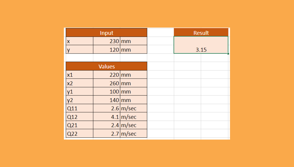
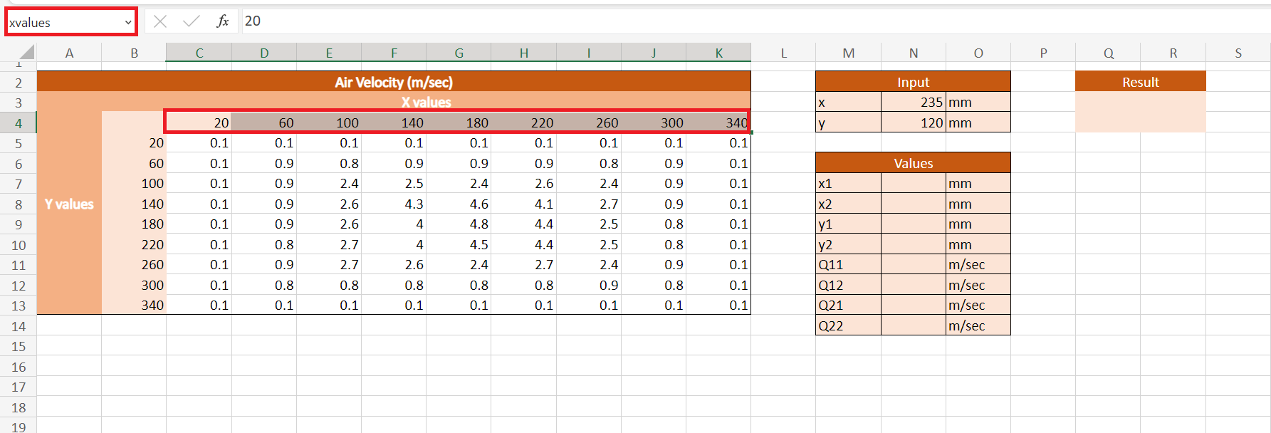
Let’s say we want to calculate the air velocity that is dependent on the horizontal position (x) and the vertical position (y). Our initial data set would look like this:

To find the estimate of the air velocity for an x-value of 230 and a y-value of 120, we need to add these values to our worksheet in the input section. 

Thus, the z-value for x=230 and y=120 will be somewhere in between the highlighted values below.  

Finding the x and y values

Since bilinear interpolation has a complicated formula, we will use the INDEX function and the MATCH function to find the x1, x2, y1, y2, and the Q values to fill in the values table. 

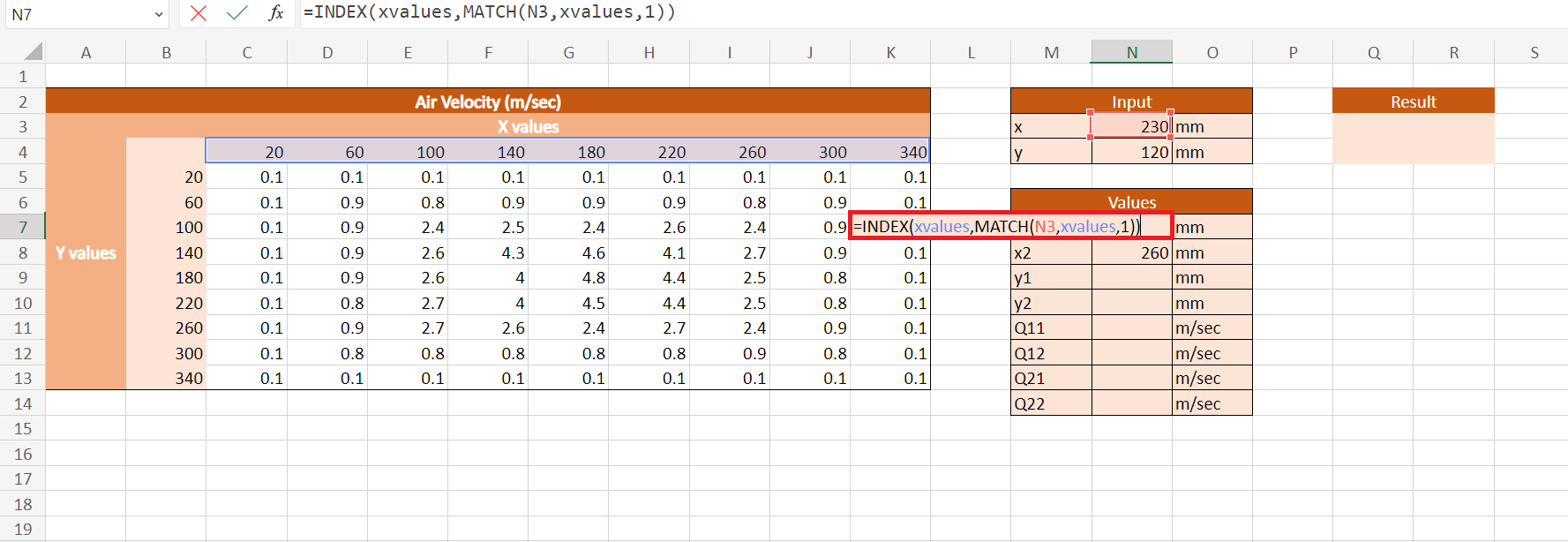
First, we will find the x1 and x2 values. The x1 value is the value in the table that is just below our desired x-value of 230, and the x2 value is just above the desired value, which is 260.

We will use the formula below to find the x1 value:

=INDEX(xvalues,MATCH(N3,xvalues,1))

The first part of the formula tells the INDEX function to search within the x-values array that was defined. Then, the MATCH function searches for the value nearest to the x-value that does not exceed our last argument, which is 1.

We will use the formula below to find the x2 value:

=INDEX(xvalues,MATCH(N3,xvalues,1)+1)

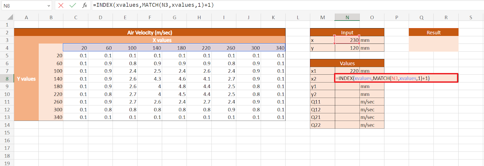
The formula for x2 will be almost the same. However, we will add a +1 at the end of the MATCH function. This will cause the position that the INDEX function looks in to be one more than the x1 position. 

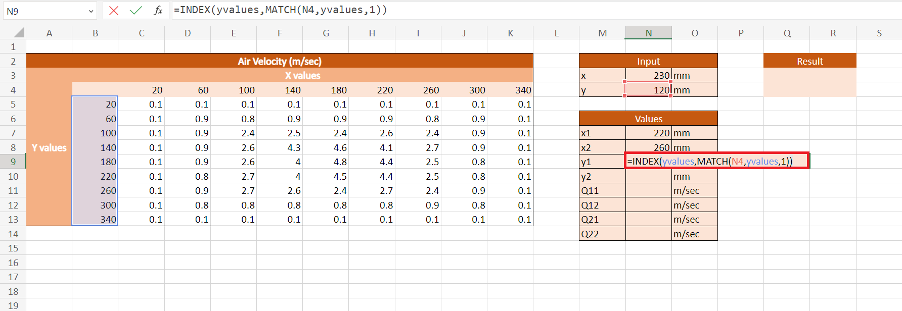
The formulas for y1 and y2 will be done in a similar way. For the y1 value, we will use the formula:

=INDEX(yvalues,MATCH(N4,yvalues,1))

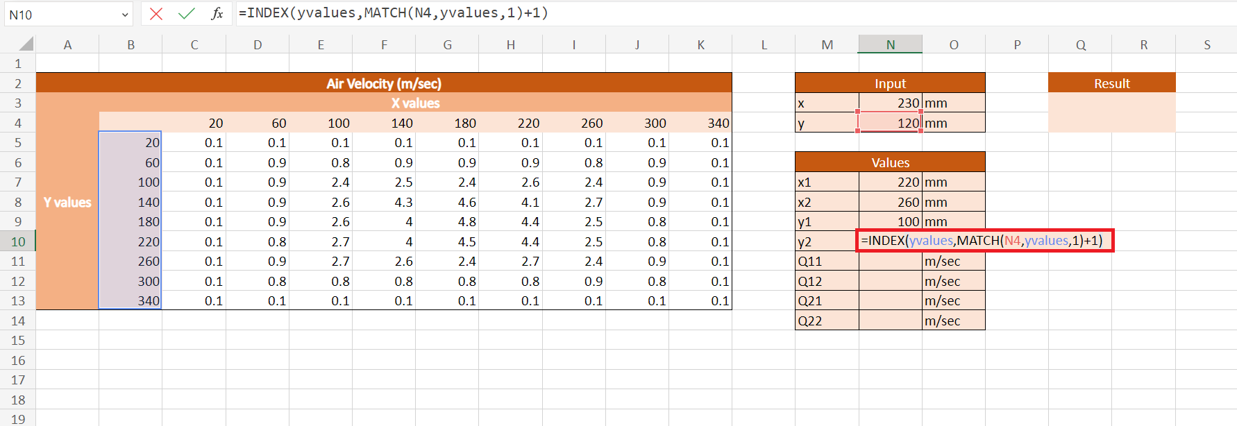
For the y2 value, we will apply this formula:

=INDEX(yvalues,MATCH(N4,yvalues,1)+1)

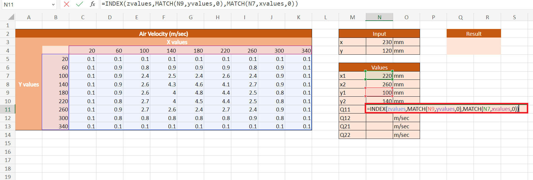
Finding the Q values

Lastly, we need to find the Q values. The Q values are actually z-values (the dependent variable in the middle of the air velocity data table).

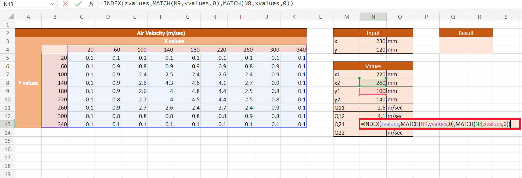
To find the Q11 value, we will utilize the formula:

=INDEX(zvalues,MATCH(N9,yvalues,0),MATCH(N7,xvalues,0))

The first argument tells the INDEX function what array to look in, which is the z-values array. 

The next argument tells the INDEX function the vertical position in the z-values array with an exact match to y_1. 

Next, the third argument tells the INDEX function the horizontal position with an exact match to x1. 

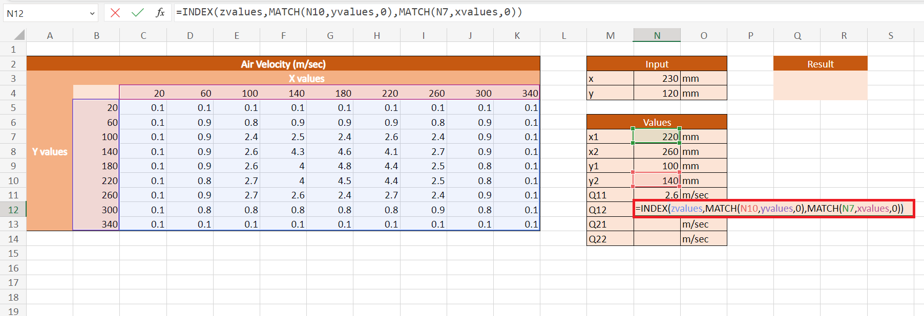
The rest of the Q values can be found using a similar formula. You can use the formula for Q12:

=INDEX(zvalues,MATCH(N10,yvalues,0),MATCH(N7,xvalues,0))

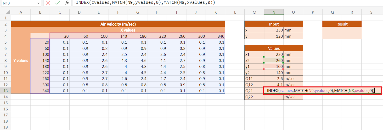
For Q21:

=INDEX(zvalues,MATCH(N9,yvalues,0),MATCH(N8,xvalues,0))

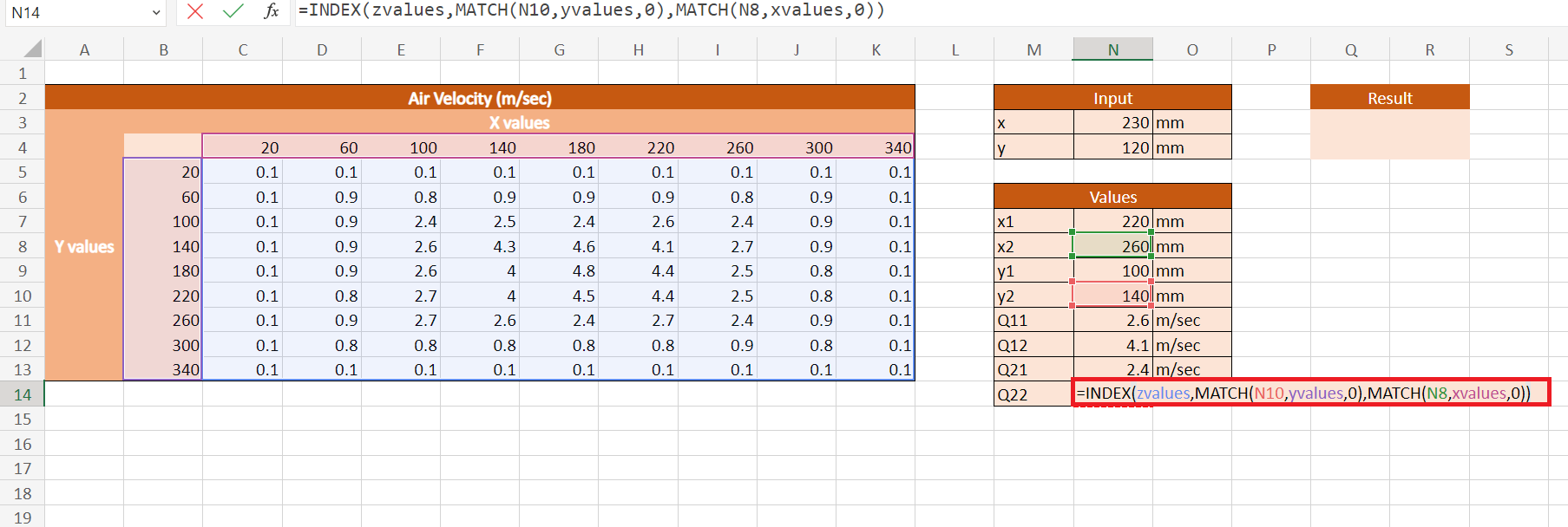
For Q22:

=INDEX(zvalues,MATCH(N10,yvalues,0),MATCH(N8,xvalues,0))

Doing Bilinear Interpolation 

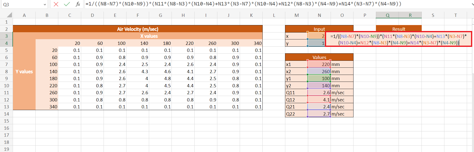
The last step is to enter the values in the bilinear interpolation formula, which is:

=1/((x_2-x_1)*(y_2-y_1))*(Q_11*(x_2-x)*(y_2-y)+Q_21*(x-x_1)*(y_2-y)+Q_12*(x_2-x)*(y-y_1)+Q_22*(x-x_1)*(y-y_1))

The final formula with our values would be:

=1/((N8-N7)*(N10-N9))*(N11*(N8-N3)*(N10-N4)+N13*(N3-N7)*(N10-N4)+N12*(N8-N3)*(N4-N9)+N14*(N3-N7)*(N4-N9))

Our final data set would look like this:

You can make your own copy of the spreadsheet above using the link below. 

Amazing! Now we can dive into the steps of doing bilinear interpolation in Excel.

How to Do Bilinear Interpolation in Excel

1. First, we will name the cell containing the x and y values in the data table. To do this, we can simply select the row containing the x-values. Then, we will go to the name box to the left of the formula bar and input “xvalues”.

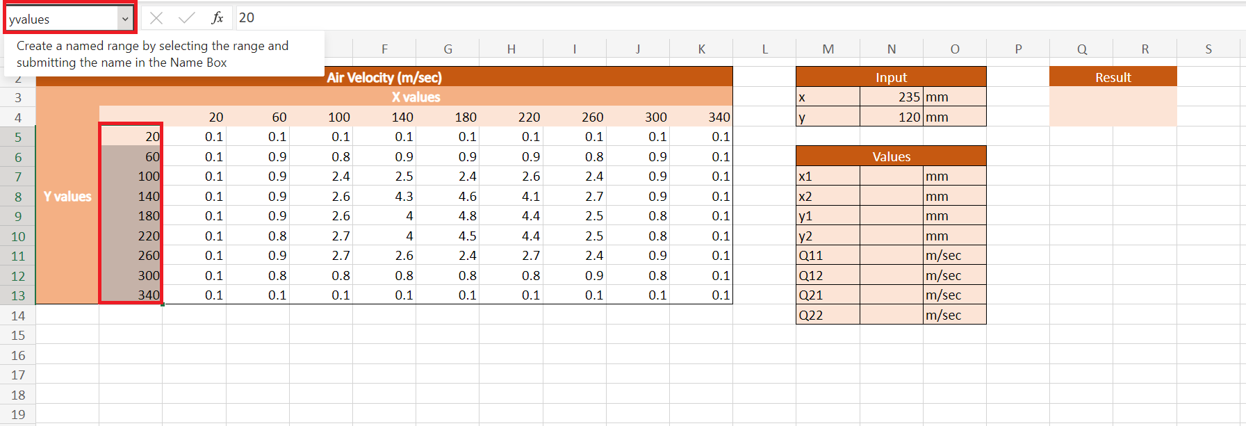
2. We will do the same to the y-values. We will select the row containing the y-values and name the row “yvalues”.

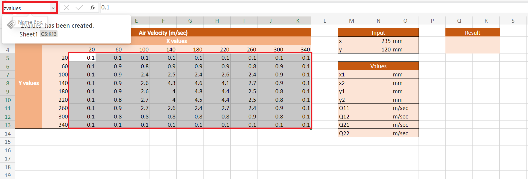
3. Then, we will select the table containing the air velocity numbers and name it “zvalues”.

4. Next, we will find the x1 value. To do this, we will use the formula “=INDEX(xvalues,MATCH(N3,xvalues,1))”. 

5. Similarly, we will use the formula “=INDEX(xvalues,MATCH(N3,xvalues,1)+1)” to find the x2 value. 

6. To find the y1 value, we will apply the formula “=INDEX(yvalues,MATCH(N4,yvalues,1))”. 

7. Then, we will use the formula “=INDEX(yvalues,MATCH(N4,yvalues,1)+1)” to find the y2 value.

8. Next, we will look for the Q values. First, we will find the Q11 value using the formula “=INDEX(zvalues,MATCH(N9,yvalues,0),MATCH(N7,xvalues,0))”.

9. Next, we will find Q12 using the formula “=INDEX(zvalues,MATCH(N10,yvalues,0),MATCH(N7,xvalues,0))”. 

10. To find Q21, we will use the formula “=INDEX(zvalues,MATCH(N9,yvalues,0),MATCH(N8,xvalues,0))”.

11. To find Q22, we will apply the formula “=INDEX(zvalues,MATCH(N10,yvalues,0),MATCH(N8,xvalues,0))”.

12. Finally, we will calculate the bilinear interpolation using all the calculated values. Our final formula would be “=1/((N8-N7)*(N10-N9))*(N11*(N8-N3)*(N10-N4)+N13*(N3-N7)*(N10-N4)+N12*(N8-N3)*(N4-N9)+N14*(N3-N7)*(N4-N9))”.

13. Press the Enter key to return the result.

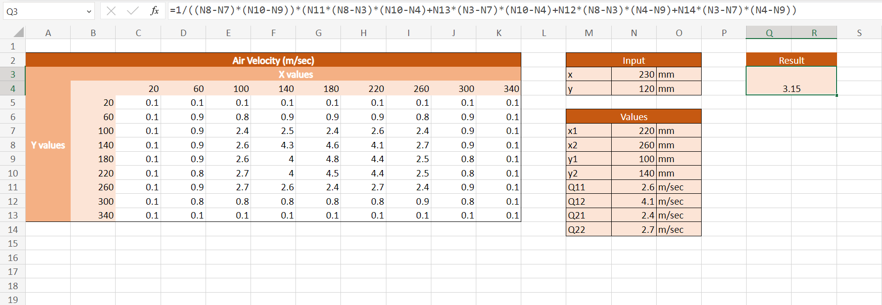
And tada! We have successfully done bilinear interpolation in Excel.

You can apply this guide whenever you need to estimate values involving three variables. You can now use the INDEX and MATCH functions and the various other Microsoft Excel formulas available to create great worksheets that work for you.

That’s pretty much it! Make sure to subscribe to our newsletter to be the first to know about the latest guides and tutorials from us.