How To Use FACTDOUBLE Function in Google Sheets

The FACTDOUBLE function in Google Sheets helps you quickly calculate the return of the double factorial of a given number.

Here are the rules for using the FACTDOUBLE function in Google Sheets:

• The function only requires the ‘value’ as an argument.
• The reference value is multiplied by its integer value that decrements by 2. 
• The decimal part of the value or reference value must be truncated before the FACTDOUBLEoperation.
• The double factorial of either positive odd or even numbers is the total product of all odd or even numbers.
• If the number is 0 and -1, the double factorial is 1.
• Any number less than -1, the value of the double factorial is undefined.

Let’s solve an example problem using a FACTDOUBLEfunction in Google Sheets.

Find the FACTDOUBLE value of the following:

Given:

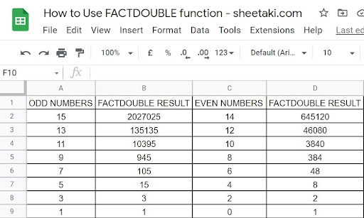
Odd number: 9

Even number: 10

Answer:

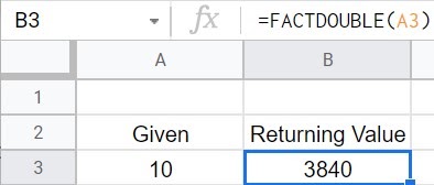
To find the returning value of the odd number 9, we must compute it like this:

9x7x5x3x1

The total product of all odd numbers from the reference value 9 to the end value 1 is 945.

Now, let’s try solving the even number, 10.

10x8x6x4x2

The process is similar to finding the returning value of the odd number. The total product of all even numbers is 3,840.

Let us now cross-check the returning value using our FACTDOUBLEfunction. 

For an odd number, 9:

For even number, 10:

The Anatomy of the FACTDOUBLE Function

Writing the syntax of the FACTDOUBLE function is not complicated. The syntax of the function is this:

After getting the gist of writing the FACTDOUBLE function, let us now understand its parts.

• = will start your FACTDOUBLE function. This informs Google Sheet that what you are writing is a function. 
• FACTDOUBLE() is our Google Sheets’ FACTDOUBLE function which gives us the double factorial value of odd or even numbers.
• Value refers to the given source or reference number of the FACTDOUBLE function.

When writing the formula, you can either substitute the ‘value’ through the actual reference number or substitute it with the specific cell where the source value was keyed in.

Example:

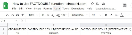
Using the same sample problem, we can write the syntax for fact double like these:

Regardless of how you write the syntax, both ways will still yield the same returning value.

A Real Example of Using FACTDOUBLE Function 

Let’s check another example below where the FACTDOUBLE function in Google Sheets is used.

In the example below, we need to put the given value and substitute it to the FACTDOUBLE formula. 

Here are the actual ways on how you write the FACTDOUBLE function. First, we can substitute the ‘value’ by using the cell of the reference value.

Now, let’s get started.

In the example above,  the function was written as ‘=FACTDOUBLE(A3)’, where ‘A3’ is the cell of the reference value.

The second way of writing the FACTDOUBLE function is by substituting the ‘value’ with the ‘reference value’ itself. 

In the second example above, the function was written as ‘=FACTDOUBLE(15)’, where ‘15’ is referred to as the reference value. 

Let us check the answers.

Regardless of how you write the formula, it will yield the same result as long as the argument you keyed in contains a valid value. 

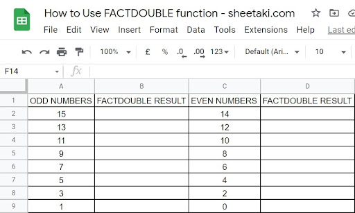
Now, let us compute the double factorial of the given odd and even numbers.

Important Things to Consider When Using the FACTDOUBLE Function

Here’s how it looks at invalid input values and computes them through the FACTDOUBLE function. 

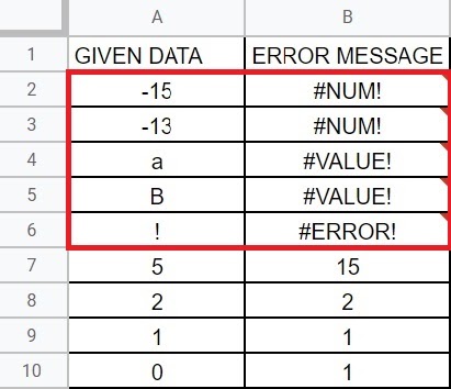
In the example above, we tried putting all possible invalid values before we computed its double factorial. The results show the following:

• Although the example above only shows negative odd numbers, the same rule applies to the negative even numbers. The double factorial results of negative odd or negative even numbers will yield a ‘#NUM!’ error message.
• Non-numeric characters (letters) – if we input lowercase or uppercase non-numeric characters as the ‘value’ of the FACTDOUBLE function, the returning value will always be an error message ‘#VALUE!’
• Non-numeric characters (punctuation marks) – if you enter any punctuation mark, use it to substitute it as your FACTDOUBLE function’s ‘value.’ The returning value will be the ‘#ERROR!’ message. 

The error messages that we pulled through different values reminded us that the FACTDOUBLE function only works with numerical values equal to or greater than 0 to n, where ‘n’ represents the positive integer.

Now, let us check the rules on how the FACTDOUBLE computes values with decimal points.

All positive numbers yield a valid returning value through decimal parts in the example above. When the function calculates the double factorial of the numbers above, the function automatically drops the decimal. See the example below.

The example above means that the function will not round the numbers to the nearest integer, but the decimal will instead be dropped entirely, leaving the integer as the ‘Value.’ 

Now that you already know how to write and compute the FACTDOUBLE function in Google Sheets, we will teach you how to use it. Kindly click on the link below to make a copy of the sample spreadsheet.

Now, let’s get started.

How to Use FACTDOUBLEFunction in Google Sheets

1. Firstly, always prepare your data. Input all given data on a blank spreadsheet.
2. Secondly, start writing the function once all the data are keyed in.

Any Google Sheets spreadsheet function always starts with an ‘=’ sign followed by the function. In today’s topic, our Google Sheet function is the FACTDOUBLE.

3. After adding the function and an open parenthesis ‘(, ‘we will now add the ‘value.’ 

Note: The ‘value’ can be substituted by the reference value’s cell or the reference value itself.

4. The picture below used the reference value’s cell, ‘A2’ followed by a closing parenthesis ‘)’ to complete the formula. 

5. Lastly, to generate the returning value, we must press the ‘ENTER’ key on our keyboard. 

6. As a result, here’s how it looks now.

Frequently Asked Questions

What happens if you input alphanumeric characters as the value to be computed? 

An error message ‘#VALUE!’ will show up. Google Sheet will read the alphanumeric characters as a text, which are invalid values.

In conclusion, the returning values of the FACTDOUBLE function depend on its given value. That is to say, that if the value is odd, the function will compute all the odd numbers starting from the given value to 1. However, though the process is the same for odd and even numbers, it computes the latter from its given value to zero. In addition to that, for the returning value to be valid, you must input a valid number and not a non-numeric or alphanumeric number.

And that’s the simplified FACTDOUBLE function in Google Sheets. If you want more Google Sheets functions and tips, you can check our website sheetaki.com for more Google Sheets formulas.

Make sure that you won’t miss anything, click the ” tab for more Google Sheets tutorial updates.

Get emails from us about Google Sheets.

Our goal this year is to create lots of rich, bite-sized tutorials for Google Sheets users like you. If you liked this one, you'll love what we are working on! Readers receive ✨ early access ✨ to new content.

Subscribe