How to Fix MATCH Function Not Working in Excel

This guide will explain how to fix errors that may occur when using the MATCH function in Excel.

Excel’s MATCH function allows you to search for a specific value in a range of cells and return the relative position of that value. For example, given a column of countries sorted by population in ascending order, we can use MATCH to locate the position of a country in the column.

You may encounter errors when using MATCH in your spreadsheet. Specifically, if the lookup value does not appear in the lookup array, the MATCH function will return a #N/A error. 

If you are certain that the value exists in the array, the problem may be with your lookup value. Possible issues include a mismatch with data types, hidden spaces or the presence of unexpected characters. 

In this guide, we will list the types of errors that may occur when using the MATCH function. We will then provide a step-by-step guide on the solutions to resolve these errors.

Real Examples of MATCH Function Not Working in Excel

Let’s explore a few examples where the MATCH function is not working as intended in Excel.

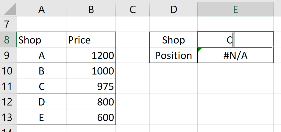
In the table above, we have a lookup table containing shop names (written here by their stall number) sorted in descending order by the average price of their products. In cell E1, the user can write the name of a shop and the shop’s position should be returned in cell E2.

We can return the shop position using the following MATCH formula:

=MATCH(E1,A2:A6,0)

In the formula above, our lookup value (the value we want to search for) is a cell reference to E1. Our formula’s lookup array (the range we want to search through) is the range A2:A6. The third argument is set to 0 to indicate we are only interested in exact matches.

However, our formula returns a #N/A error instead of the correct position of 3. There are several reasons why this may occur.

First, we must identify whether the lookup value is formatted as the same data type as the lookup array. If the lookup value is stored as a number and the lookup array stores the shop names as text, our formula will not find an exact match.

We can fix this issue by converting our lookup value into the right data type.

• If we want to convert our lookup value from a text to a number, we can add a double negative sign:
  

  =MATCH(--E1, A2:A6, 0)

• If we want to convert our lookup value to text, we can append an empty string:
  

  =MATCH(E1&””, A2:6, 0)

Another reason why the MATCH function cannot find an exact match is the presence of unexpected characters. 

For example, given a lookup value of “ 34 “, the MATCH function will not be able to return a match with the value “34” in the lookup array. Similarly, unneeded line breaks and non-printing characters may prevent the MATCH function from working correctly.

In the image above, our lookup value in cell K8 has an extra line break that may prevent our MATCH function from finding an exact match.

• We can strip away unneeded line breaks using the following formula:
  

  =MATCH(CLEAN(K8),G9:G13,0)

• If our lookup values contain trailing or leading spaces, we can use the TRIM function instead:
  

  =MATCH(TRIM(K8),G9:G13,0)

Your formula may also return a #NAME? error, which occurs when using a function that does not exist. This typically occurs when the user misspells the name of the function.

Click on the link below to create your own copy of our examples. 

Head to the next section to read our step-by-step tutorial on how to fix cases where the MATCH function is not working in Excel.

How to Fix MATCH Function Not Working in Excel

1. The MATCH function may be returning a #N/A error because your lookup value is formatted incorrectly. Excel may place a green marker on the upper-left corner of your cell to flag this type of error.
   Clicking on the alert symbol will give you the option to convert the value to the appropriate data type.
   
2. We can also format the value manually using the Number Format dropdown menu in the Home tab.
   
3. Once the data types of the lookup value and lookup array are matching, the MATCH function will work as intended.
   
4. If our lookup value is stored as a number and our lookup array is stored as text, we can append an empty string to convert our lookup value into text.
   In the image above, we used the formula =MATCH(E1&””,A2:A6,0) to convert the number 26 into the string “26”.
   
5. If the lookup value is stored as text and we want to convert it to a number, we can add a double negative sign (–) before the lookup value in our formula.
   In the image above, we used the formula =MATCH(–E8,A9:A13,0) to convert the string “26” into a number.
   
6. Another reason why the MATCH function returns a #N/A error is because of unexpected characters such as a leading or trailing space.
   Removing these unneeded characters from your lookup value will allow the function to match values properly.
   
7. We can also use the TRIM and CLEAN functions to remove unexpected characters from our lookup value.
   The TRIM function takes a string as input and removes all extra spaces found at the start and end of the string. This function also deletes spaces between words so that each word is separated by a single space.
   
   If your lookup value includes line breaks, you can use the CLEAN function instead. The CLEAN function strips both line breaks and non-printing characters from a given text.
   
8. If you encounter a #NAME? error, it is possible that you’ve misspelled the function name. You can fix this error by adding the proper function name to your formula.
   
9. The MATCH function will always return a #N/A error if the function tries to find an exact match of the lookup value and finds no results.
   We can avoid this error from showing by wrapping the formula with an IFNA function.
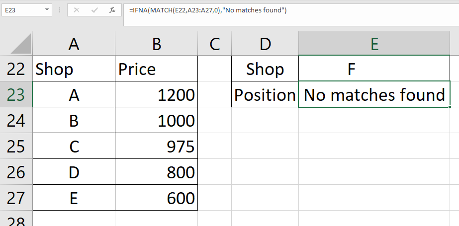   In the image above, we used the formula =IFNA(MATCH(E22, A23:A27, 0), “No matches found”) to output custom text if an exact match of the lookup value is not found.
   

These are the most common fixes you can use to troubleshoot errors that occur when using the MATCH function in Excel.

You should now understand the reasons why the MATCH function is not working. With the help of our guide, you can now troubleshoot your formula and find a solution yourself. 

If you want to learn more about fixing similar lookup formulas, read our guide on how to fix INDEX-MATCH function not working in Excel.

That’s all for now!  Be sure to check out our library of spreadsheet resources, tips, and tricks! 

Get emails from us about Excel.

Our goal this year is to create lots of rich, bite-sized tutorials for Excel users like you. If you liked this one, you'd love what we are working on! Readers receive early access to new content.

Subscribe