How to Use MATCH Function in Excel

The MATCH function in Excel is useful when you need to give the relative position of an item within a range of cells.

This function is commonly used along with the INDEX function to create a powerful lookup formula. 

The rules for using the MATCH function in Excel are as follows:

• The function requires a search key, range, and search type.
• The function then outputs the relative position of an item specified by the given parameters.

Let’s take a look at a quick example where we can use the MATCH function. in Excel

We have a list of values in ascending order, and we have a value to search for in this range. For example, in an array of ages, we want to know whether anyone is aged 30. Afterward, we want to know what position that person is on the list.

 Is it possible to get the position of the value that matches what we’re searching for?

With the MATCH function, it becomes quite easy to get the relative position of a matched value. The MATCH function can also be used along with the INDEX function to provide a VLOOKUP functionality that is not restricted to matching with the first column of a table.

Now that we know when to use the MATCH function in Excel, let’s dive into how to use it and work on an actual sample spreadsheet.

The Anatomy of the MATCH Function

The syntax of the MATCH function in Excel is as follows:

=MATCH(lookup_value, lookup_array, [match_type])

Let’s dissect this formula and understand what each of these terms means:

• = the equal sign is how we start any given function in Excel.
• MATCH() is our MATCH function. It returns the relative position of an item in a range.
• lookup_value refers to the value that you want to match in lookup_array. The lookup value can be a value or a cell reference.
• lookup_array refers to the range of cells being searched
• match_type refers to how Excel matches lookup_value with the range of values in lookup_array. By default, this argument is set to 1.
• A match_type of 1 indicates that MATCH will find the largest value that is less than or equal to the lookup_value.
• A match_type equal to 0 indicates that MATCH will find the first value that is exactly equal to the lookup_value.
• Having a match_type of -1 indicates that MATCH will find the smallest value that is greater than or equal to the lookup value.

A Real Example of Using MATCH Function

Let’s take a look at a real example of the MATCH function being used in an Excel spreadsheet.

In the example below, we have a table of different raw meats as well as the amount in kilograms we have available. The MATCH formula in row 8 searches for a cell in the range B2:B5 that is equal to 11. The formula correctly indicates that the 2nd row in the range equals 11.

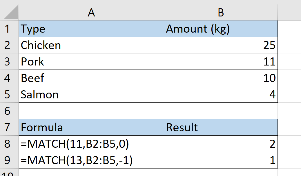
The MATCH function in row 9 uses a different method of search. In this formula, we’re looking for the lowest value in the range B2:B5, which is greater than or equal to the value of 13. This leaves us with 25, which is the 1st value in the range.

In the example below, we have another list of items. The list is now arranged in ascending order this time. In our first MATCH formula, we tried to find an exact match of 100. Since no matches were found, the formula returned an error. In the second MATCH formula, we searched for the highest value less than or equal to 50. Our formula returns the value of 2, which points to the 2nd value in our range.

You can make your own copy of the spreadsheet above using the link attached below. 

If you’re ready to try out the MATCH function in Excel, let’s begin writing it ourselves!

How to Use MATCH Function in Excel

This section will guide you through each step needed to start using the MATCH function in Excel. You’ll learn how we can use the MATCH function to get the relative position of an item that matches a provided lookup value.

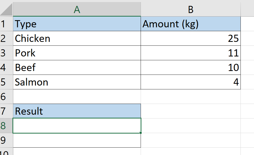
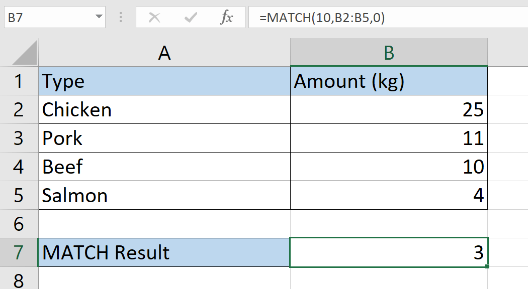
1. First, select the cell where we will place our MATCH function. In this example, we’ll place the formula in cell A8.
   
   
   
2. Next, we just simply type the equal sign ‘=‘ to begin the function, followed by the string ‘MATCH(‘.
   
   
   
3. Fill in the arguments of the MATCH function. In the example below, we specified a lookup value of 10, a lookup range of B2:B5, and a search mode of 0 (which works for descending values in a range).
   

In the next part of this guide, we’ll briefly explore how you can use the MATCH and INDEX functions together.

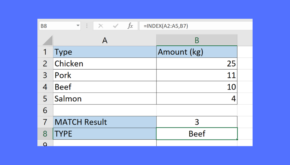
1. We can use the INDEX function to return a specific value in the same row as the matched value. In this example, we want to return the corresponding value in column A. We simply have to specify the range A2:A5 and the result of our MATCH function.
   
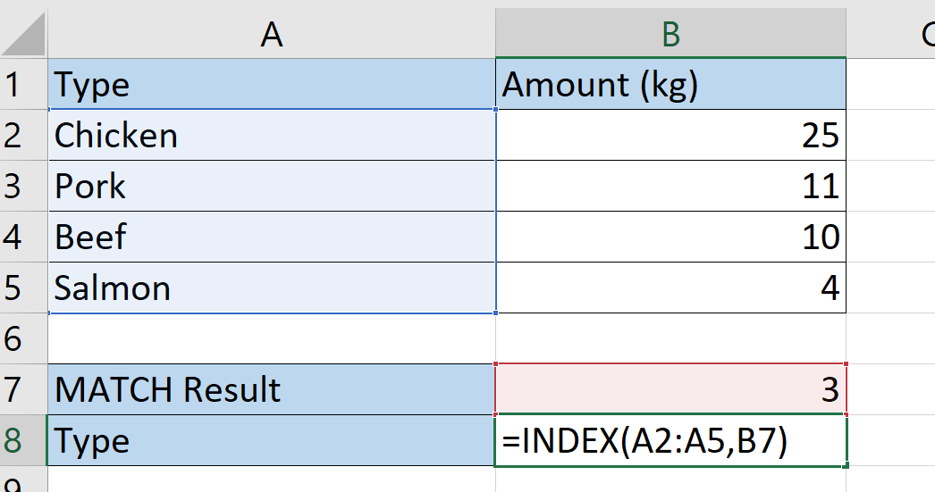
2. Hit the Enter key to evaluate the function. We now returned the corresponding type of the amount we matched with.
   
   

Frequently Asked Questions (FAQ)

1. Why does my MATCH formula return an error?
   If the MATCH function fails to find a match in the provided range, the function will return a #N/A error.
2. Is the MATCH formula case-sensitive?
   The MATCH function does not distinguish between uppercase and lowercase letters. You also have the option to use wildcard characters such as the “?” and “*” symbols. The question mark matches any single character, while an asterisk matches any sequence of characters.

That should be everything you need to remember when working with the MATCH function in Excel. This step-by-step guide shows how simple it is to search and get the relative position of a value in a given range.

The MATCH function is just one example of a useful function in  Microsoft Excel. With so many other Excel functions out there, there will be plenty of options for you to create more powerful worksheets.

Are you interested in learning more about what Excel can do? Make sure to subscribe to our newsletter to be the first to know about the latest guides and tutorials from us.

Get emails from us about Excel.

Our goal this year is to create lots of rich, bite-sized tutorials for Excel users like you. If you liked this one, you'd love what we are working on! Readers receive ✨ early access ✨ to new content.

Subscribe