This guide will explain how to forecast cash flow in Excel.
A forecast cash flow is a useful tool used by companies to track their financial performance in real-time. So it compares the projected or expected cash flow and the company’s actual cash flow.
And this is usually made to forecast the fiscal year or a 12-month forecast cash flow. Basically, it will forecast the company’s cash flow in real-time for the entire year or for 12 months.
So cash flow refers to the cash or money that comes in or out of the company. Essentially, the movement of cash in the company.
Furthermore, Excel is a useful tool for creating a forecast cash flow. Since it has the necessary functions and features, it will make the process easier.
Let’s take an example.
Suppose you are the finance head of your company. So you are expected to create a forecast cash flow of the company for the year 2022. And to make this task easier, you will create the forecast cash flow in Excel.
Great! Let’s check a real example of forecasting cash flow in Excel.
A Real Example of Forecasting Cash Flow in Excel
There are many components to prepare in creating a forecast cash flow in Excel.
Firstly, we must prepare a list of the company’s cash flow drivers. So cash flow drivers are things or activities that generate cash for the company. Basically, anything that earns or gives money to the company.
In this case, we will list out the company cash flow drivers. And we will be using previous data to create an assumption on how much the company can earn in a year. Additionally, the more data we have, the more realistic our forecast will be.
Next, we will continuously update the forecast cash flow in Excel as the year goes on. Basically, we have two metrics: expected and actual performance. Furthermore, our goal should be to have little to no difference between the two metrics.
Based on our cash flow drivers and previous company data, we will input our assumptions in the expected column for each month. So each month will be divided into two columns. One is for the expected or assumed performance. And the other is for the actual performance.
On the left-most side of our forecast cash flow, we will input our expected cash receipts each month. And below that, we will have our expected costs each month.
Then, we need to prepare a column for each month to input our expected and actual performance on each category of the cash receipts and costs.
Also, we will have the total amount for the cash receipt and costs each month at the bottom. By adding the total cash receipt and costs of the month, we can get the net change in cash, which refers to how much the company’s cash balance increased or decreased in the month.
Lastly, we will calculate the monthly variance at the very bottom of the entire table. Furthermore, the variance will tell us the difference between our expected and actual performance.
Furthermore, we will prepare a separate table at the right most containing the summary of the forecast cash flow. And it will tell us the total expected and actual performance for the entire year and the variance between the total amounts.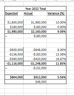
You can make your own copy of the spreadsheet above using the link attached below.
How to Forecast Cash Flow in Excel
In this section, we will discuss the step-by-step process of how forecasting cash flow in Excel.
1. Firstly, let’s create the table. In our first column, we will input all the components of our forecast cash flow, such as the cash receipts and costs. Furthermore, in the next following columns, we will input the 12 months and divide each month into two columns for our expected and actual performance.
2. Secondly, we will input all the assumptions we have per component in our expected columns. And as the year goes on, we will input the actual data per month.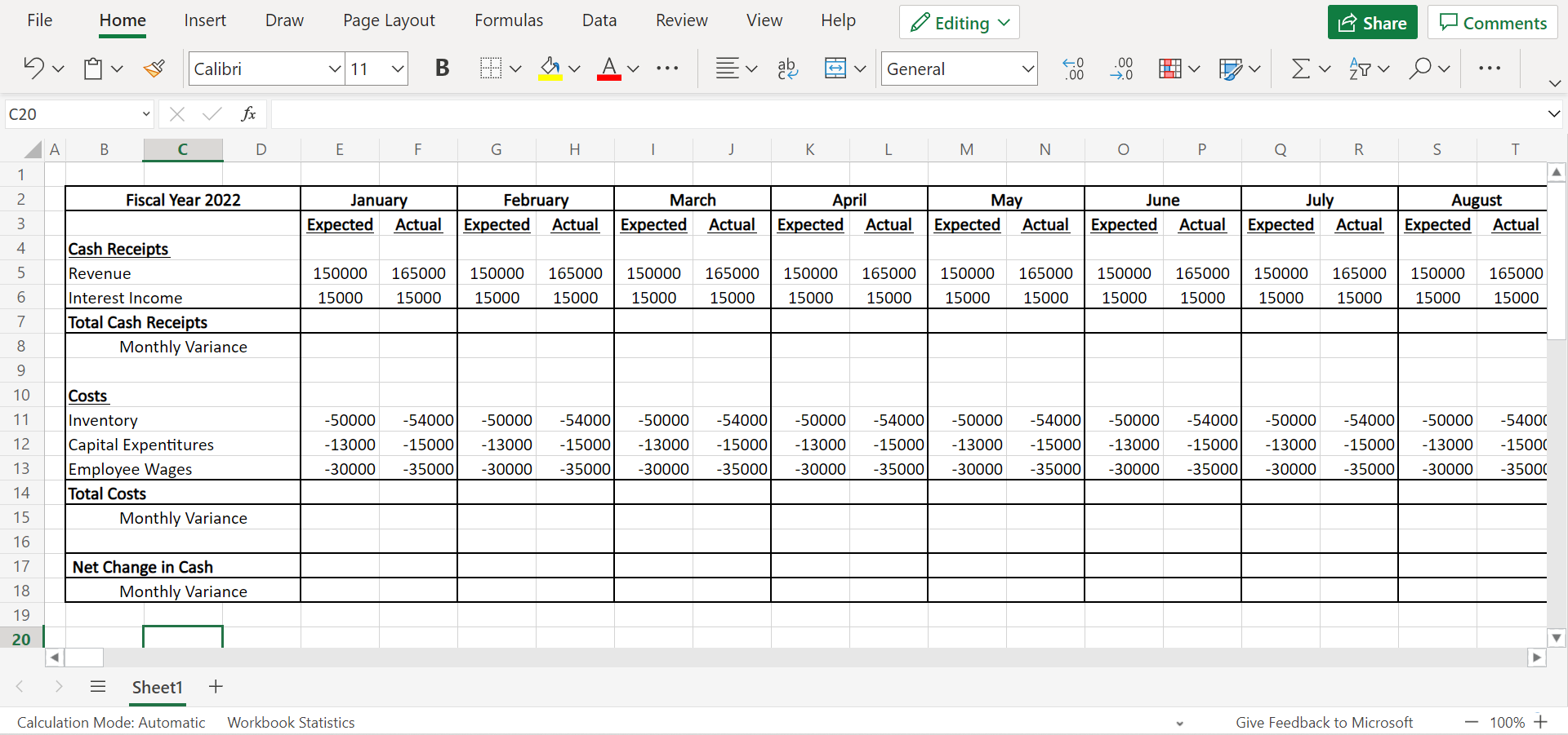
3. Before we do our calculations, let’s input a currency symbol. So select the table and right-click. Then, click Number Format.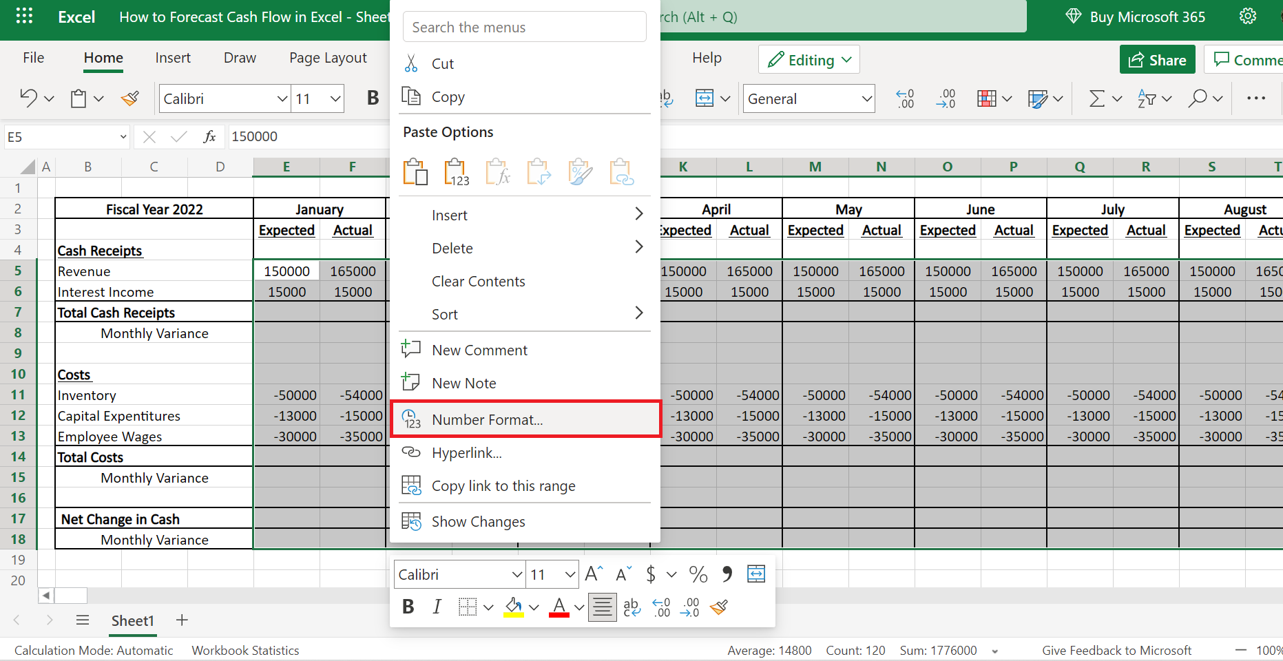
4. Then, go to the Currency category. Additionally, we can choose any currency applicable in the Symbol dropdown menu. And change the Decimal places to 0. Lastly, click OK to apply the changes.
5. And now let’s start doing calculations. To get the Total Cash Receipts, type in the formula “=SUM(E5:56)”. Next, drag the formula to copy it to the entire row. 
6. Then, we will calculate the Monthly Variance. Input the formula “=+F7-E7”. And copy the formula.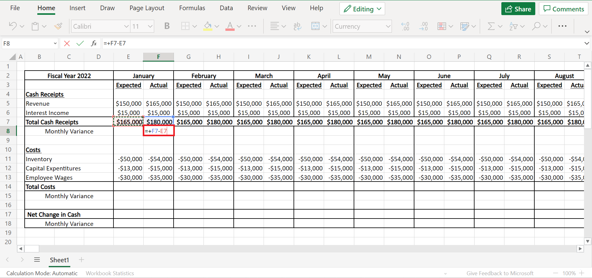
7. After copying the formula, we will paste it into the Actual column of each month. Additionally, when pasting, click the dropdown menu and select the third option, which will paste the formula. 
8. To calculate the Total Cost, type in the formula ‘=SUM(E11:E13)’. And copy the formula by dragging it to the entire row. 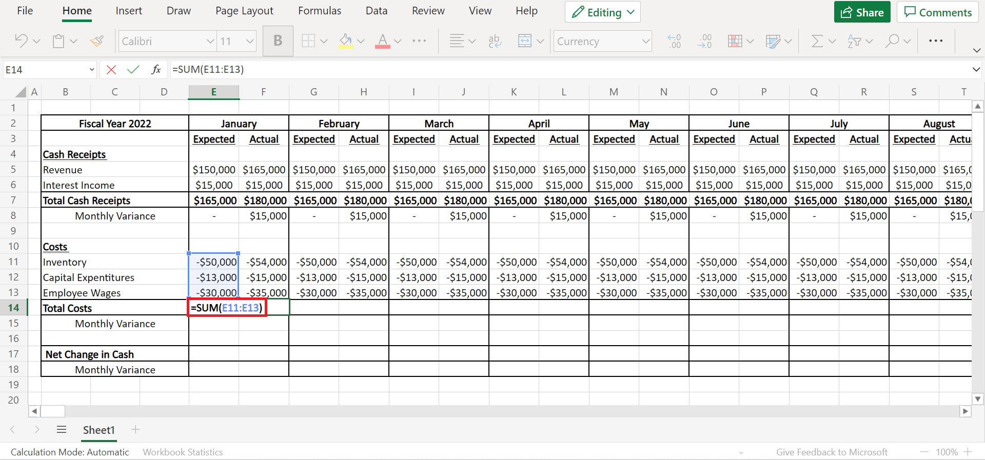
9. Next, input the formula ‘=+F14-E14’ to get the Monthly Variance of the costs. 
10. We’re almost done! Now let’s calculate the Net Change in Cash. To do this, type in the formula ‘=+SUM(E7;E14)’.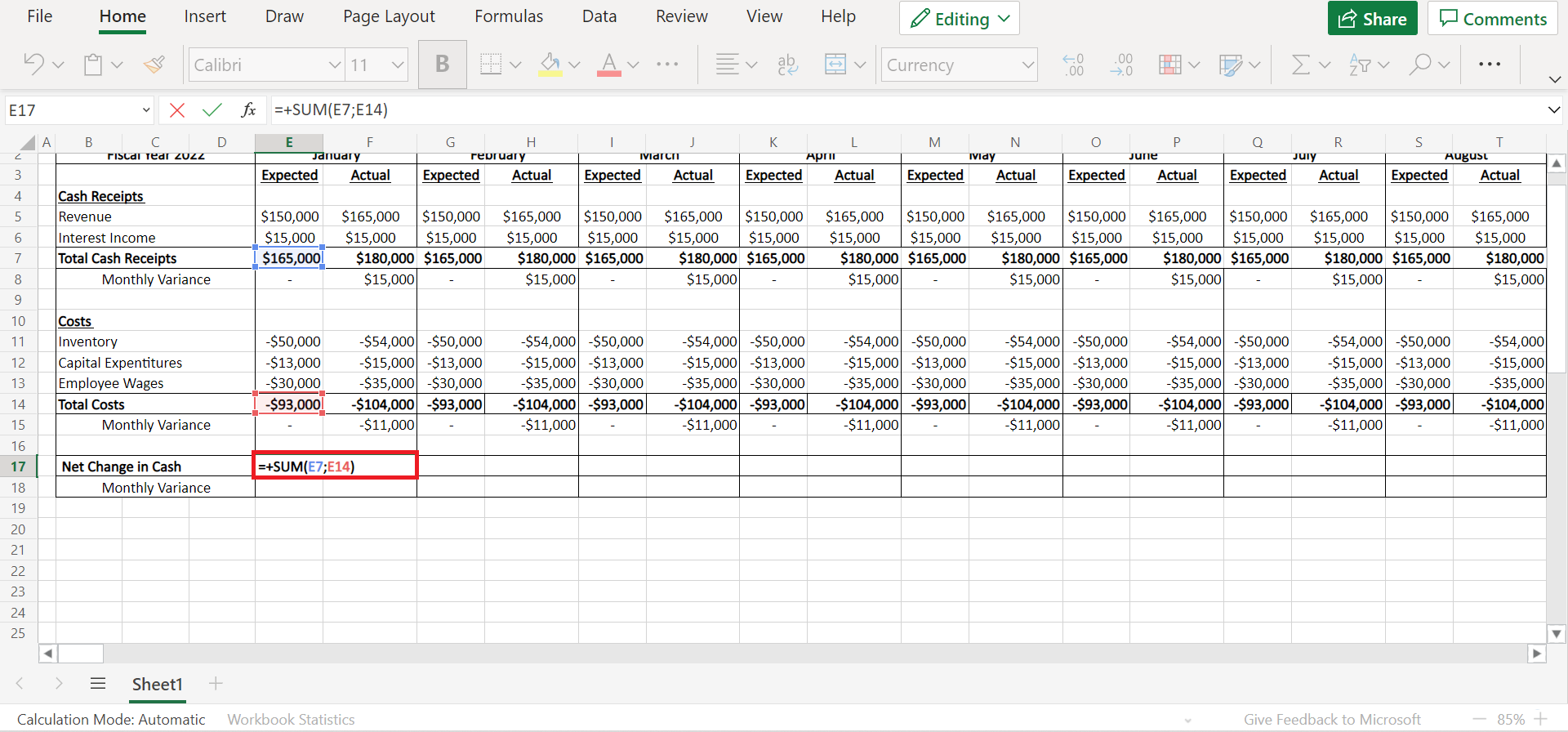
11. Lastly, let’s calculate the Monthly Variance for the net change. So input the formula ‘=+F17-E17’.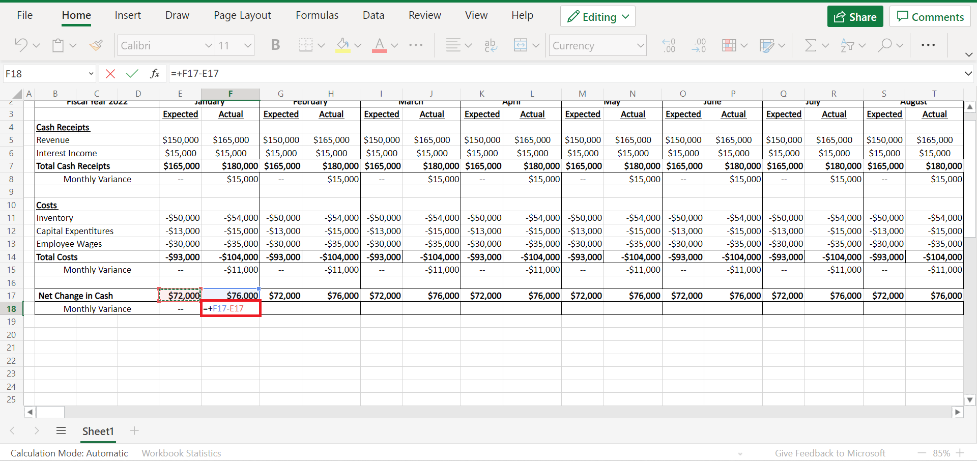
12. And we are done with the main table of our forecast cash flow in Excel.
13. Afterwards, it’s time to make the summary table of our forecast cash flow. Firstly, let’s create the table. And we only need three columns for the Expected, Actual, and Variance.
14. Next, let’s calculate the total expected performance in the entire year. So input the formula ‘SUMIF(E$3:AB$3;$AD$3;E5:AB5)’. And drag down to copy the formula to the rest of the column.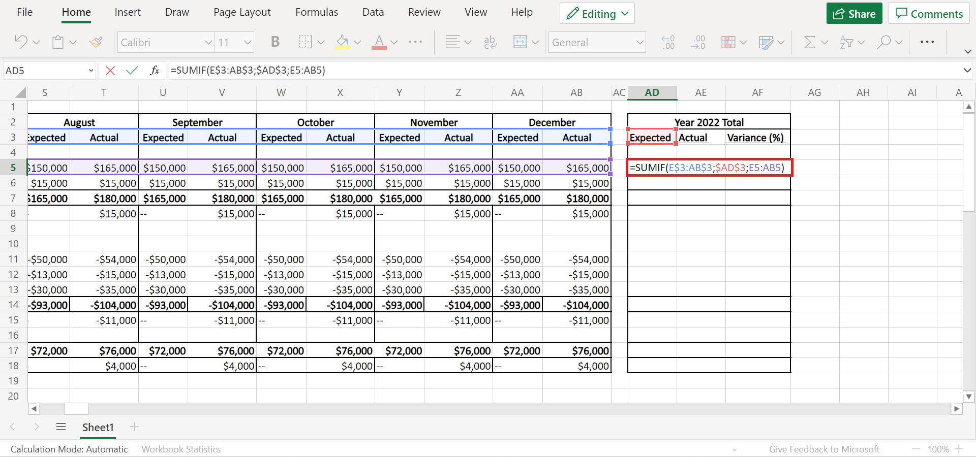
15. Then, input the formula ‘SUMIF(E$3:AB$3;$AE$3;E5:AB5)’ to get the total for the Actual column. Afterwards, drag down to copy the formula to the entire column.
16. Next, let’s calculate the percentage of the Variance. To do this, type in the formula ‘=+AE5/AD5-1’. And drag down the formula to apply to the entire column. 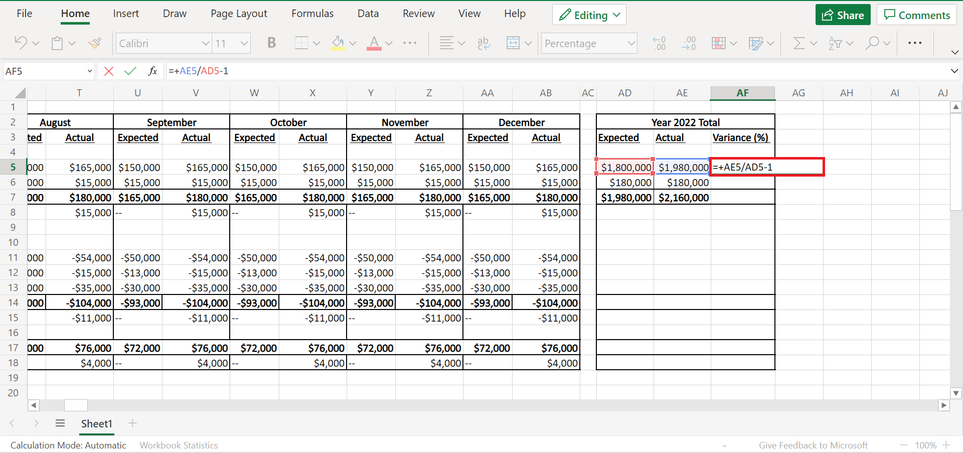
17. And tada! We have successfully learned how to forecast cash flow in Excel.
Awesome! You have learned how to forecast cash flow in Excel. Hence, you can now apply this learning in your own work.
Are you interested in learning more about what Excel can do? You can now use the various other Microsoft Excel formulas available to create great worksheets that work for you. Make sure to subscribe to our newsletter to be the first to know about the latest guides and tutorials from us.


