How to Use TEXTAFTER Function in Excel

This guide will discuss how to use the TEXTAFTER function in Excel. 

The rules for using the TEXTAFTER function in Excel are the following:

• The output from the TEXTAFTER function is a single value.
• If instance_num is blank or empty, the TEXTAFTER function will use 1 as a default.
• If match_mode is left blank or empty, the default is 0. And the TEXTAFTER function is case-sensitive.
• The TEXTAFTER function will not use the end of a text string as a delimiter by default. So match_end is 0 by default. 
• The if_not_found argument returns #N/A by default. 

So the TEXTAFTER function is used to extract a string or text after a given or specified delimiter. But, this is not to be confused with the TEXTSPLIT function. 

Essentially, the TEXTAFTER function is for extracting text or string after a delimiter, while the TEXTSPLIT function is used to extract all text separated by delimiters. Furthermore, the TEXTAFTER function can also return a text or string after the nth occurrence of a specific delimiter. 

Let’s take a sample scenario wherein we need to use the TEXTAFTER function in Excel. 

Suppose you have a class list containing the surnames and first names of each student in a class. But, you need to create a new table containing each student’s first name only. Of course, you can individually type each first name of the students. 

But, this would take too much time and effort. For efficiency, the best way to perform this task is by using the TEXTAFTER function. Because the function will automatically extract the needed values and return them separately, making your tasks easier and faster.

Great! Before we move on to a real example of how to use the TEXTAFTER function in Excel, let’s first learn how to write the function and its arguments. 

The Anatomy of the TEXTAFTER Function

The syntax or the way we write the TEXTAFTER function is as follows:

=TEXTAFTER(text, delimiter, [instance_num], [,match_mode], [match_end], [if_not_found])

Let’s take apart this formula and understand what each term means:

• = the equal sign is how we activate or start a function in Excel. 
• TEXTAFTER() is our TEXTAFTER function. And this function will return a text after a given or specified delimiting characters. 
• text is a required argument. And this refers to the text containing the delimiters that we want to extract from.
• delimiter is another required argument. And this refers to the character or string we will use as a delimiter. 
• instance_num is an optional argument. And this refers to the desired occurrence of a delimiter. By default, the instance_num is 1. Additionally, we can input a negative number to search from the end. 
• match_mode is another optional argument. And this will search the selected text for a delimiter match. By default, match_mode is case-sensitive. 
• match_end is used to decide whether to match the delimiter against the end of the text. But, they are not matched by default. Also, this is another optional argument. 
• if_not_found is an optional argument. And this refers to the value or character returned if no match is found. By default, #N/A is returned. 

Amazing! Since we have learned the syntax of the TEXTAFTER function, let’s move on to a real example of using this function. 

A Real Example of Using the TEXTAFTER Function in Excel

For instance, we have a data set containing the surname and first name of each student in a class. And we need to extract the first name of each student. Firstly, our initial data set would look like this: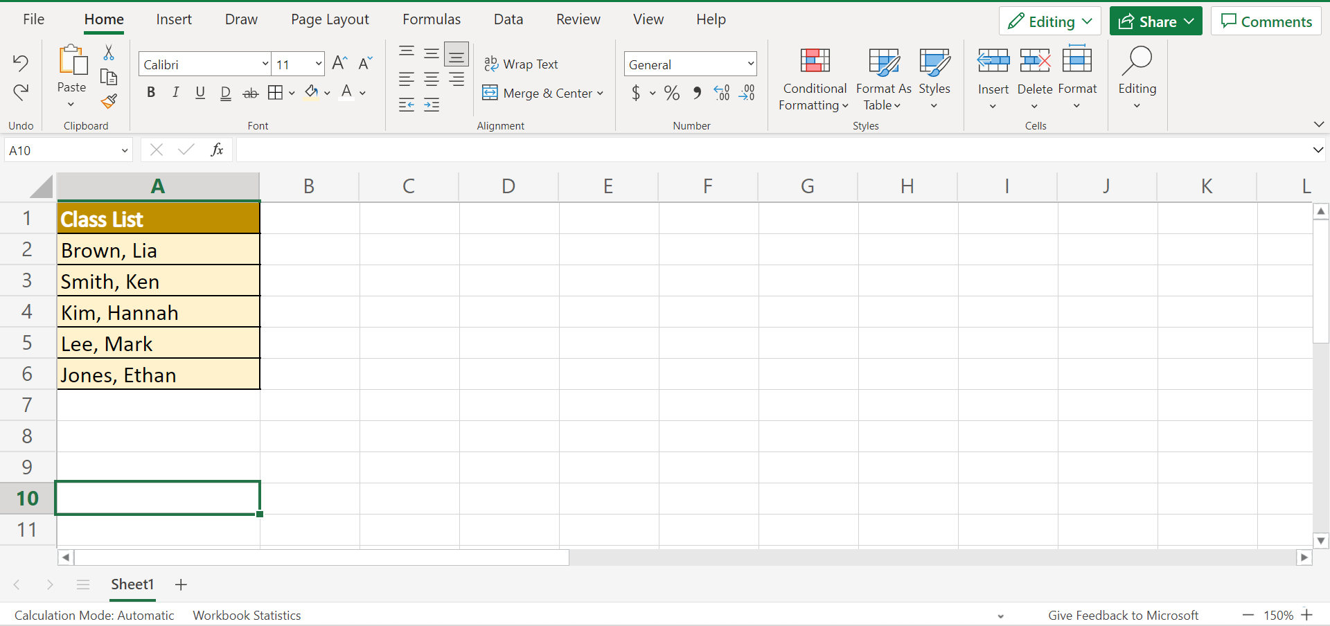

So the TEXTAFTER function would extract each student’s first name and return that value. And we only need to specify the delimiter. In this case, the surname and first name are separated by the delimiter comma. 

So the TEXTAFTER function essentially extracts what comes after the delimiter comma which in this case is the first name. And tada! We have successfully extracted the first names of the students. 

Additionally, we can also extract a text after the nth occurrence of the delimiter using the instance_num argument. For example, we want to extract only the last digit from a code. 

And we can simply do that by inputting 2 which means the TEXTAFTER function will return the text after the first and second occurrence of the specified delimiter.  

Also, the function supports negative values inputted for instance_num meaning we can return the text after the last occurrence of a delimiter. For instance, we want to return the last two groups of digits of a code. So we can input -2 in instance_num which will return the month and year. 

Finally, our data set would look like this after successfully using the TEXTAFTER function in Excel.

You can make your own copy of the spreadsheet above using the link attached below. 

Great! Now let’s dive into the process of how to use the TEXTAFTER function in Excel. 

How to Use the TEXTAFTER Function in Excel

In this section, we will explain the step-by-step process of how to use the TEXTAFTER function in Excel. Additionally, we will discuss how to utilize the different optional arguments of the function. 

1. Firstly, we will simply use the TEXTAFTER function to extract the students’ first names. To do this, type an equal sign and the function name to start the function. Then, simply input the formula “=TEXTAFTER(A2, “,”)”. Lastly, press the Enter key to return the results.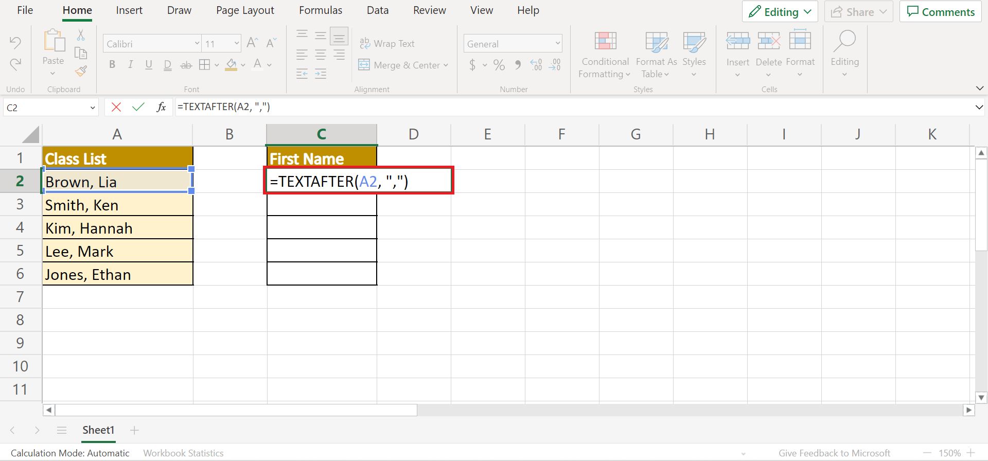

2. Next, drag down the formula to copy to the rest of the column.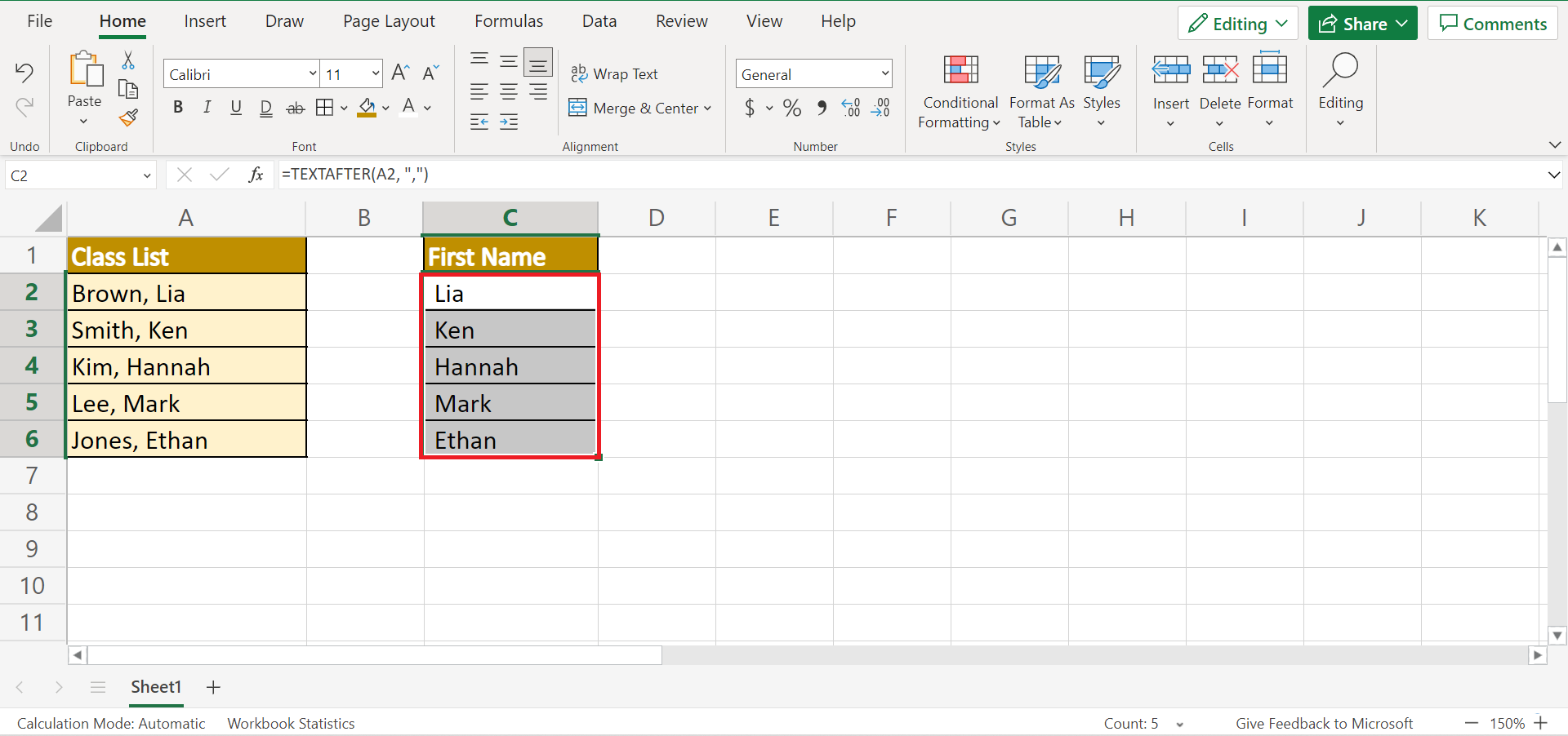

3. And tada! We have successfully used the TEXTAFTER function in Excel.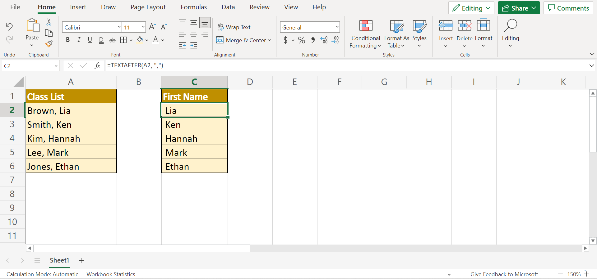

4. Next, let’s learn how to extract text after the nth occurrence of a delimiter. In this case, we will extract the last digits from the given data. To do this, we need to use the instance_num argument. In this case, the year is after 2 occurrences of the delimiter. So type in the formula “=TEXTAFTER(E2,”-“,2)”. Then, press the Enter key to return the last digits.

5. Furthermore, let’s try inputting a negative number in the instance_num argument. For example, we want to extract the data’s last two groups of digits. So we will type in the formula “=TEXTAFTER(E2,”-“,-2)”. Then, press the Enter key to return the results.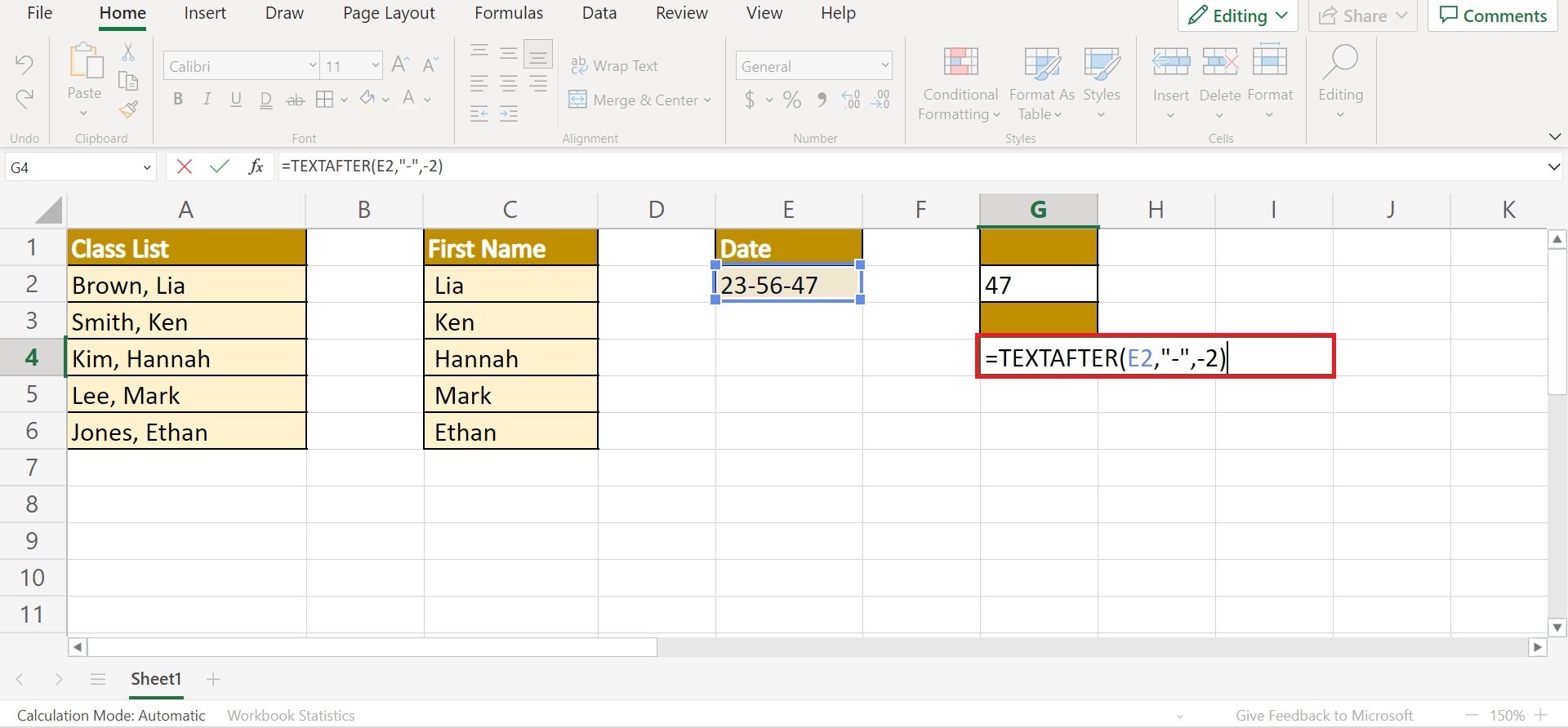

6. And tada! We have successfully used the optional arguments in the TEXTAFTER function for different purposes.

And that’s pretty much it! We have explained how to use the TEXTAFTER function in Excel. Now you can apply this learning to your work and use the different optional arguments of the function to adjust to your situation. 

Are you interested in learning more about what Excel can do? You can now use the TEXTAFTER function and the various other Microsoft Excel formulas available to create great worksheets that work for you. Make sure to subscribe to our newsletter to be the first to know about the latest guides and tutorials from us.

Get emails from us about Google Sheets.

Our goal this year is to create lots of rich, bite-sized tutorials for Google Sheets users like you. If you liked this one, you'll love what we are working on! Readers receive ✨ early access ✨ to new content.

Subscribe