


This guide will explain how you can use the ISERROR function in Excel to catch and handle errors you may encounter when using the VLOOKUP function.
If the VLOOKUP function cannot find a lookup value, it will return a #N/A error. We can use the ISERROR function to return a different result in case this error occurs.
The rules for using the ISERROR function in Excel are as follows:
- The function requires two arguments: the argument that is checked for an error, and the value to return if the formula evaluates to an error.
- The function outputs the second argument if an error is found. Otherwise, the function returns the formula’s output in the first argument.
Let’s take a look at a quick example of a scenario where we can use the IFERROR function with the VLOOKUP function.
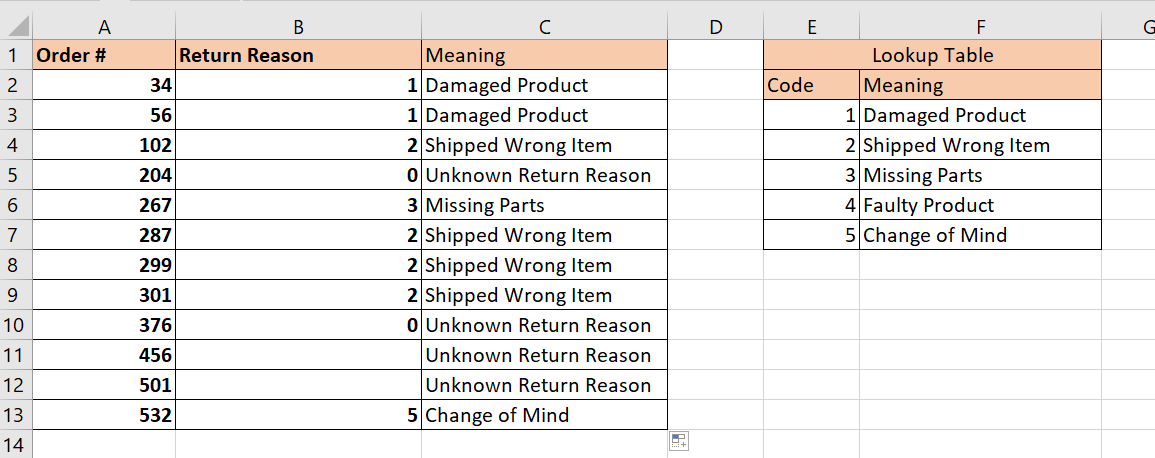
As an owner of an online business, you may encounter returned orders. Customers can return the order for various reasons, such as receiving a damaged product or an incorrect item.
The system that handles the returns process conveniently lets the customers provide a reason for the return. Each return shows up in your database in a table with the order number, date of request, and an integer with a return reason. You have made a lookup table that you use to easily convert the integer code into a human-readable status such as “Damaged Product” or “Shipped Wrong Item”.
Later on, you start receiving returns with missing return reasons. You suspect this might be a system issue. Your table is now full of #N/A errors since the lookup table you’ve set up does not have the given codes.

How can you catch these errors and provide a default string such as “Unknown Return Reason”?
We can use the ISERROR function to detect these lookup errors coming from VLOOKUP. We can simply wrap our current VLOOKUP formula with the ISERROR function to give our formula this additional functionality.
Now that we know how useful the ISERROR function is paired with the VLOOKUP function, let’s look at how it might work on an actual spreadsheet.
A Real Example of Using ISERROR with VLOOKUP
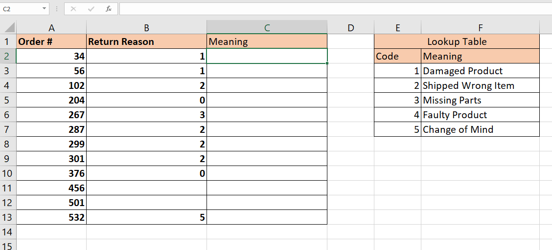
Let’s take a look at a real example of a VLOOKUP function with an ISERROR function wrapped around it.
The table below uses the ISERROR function to print out a default text string if the VLOOKUP function fails to find the lookup value.
To get the values in Column C, we just need to use the following formula:
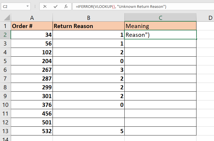
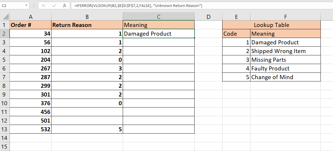
=IFERROR(VLOOKUP(B2,$E$3:$F$7,2,FALSE), "Unknown Return Reason")
The formula above uses a VLOOKUP formula to find the appropriate meaning behind each code. Our first argument B2 indicates our lookup value which we will try to find in the range E3:F7. Our second argument is written as an absolute cell range reference so we can easily drag down the formula later on.
The VLOOKUP formula now serves as the first argument of our IFERROR function. If the VLOOKUP function returns any error, the formula will return “Unknown Return Reason” instead of “#N/A”.
You can make your own copy of the spreadsheet above using the link attached below.
If you’re ready to try out the IFERROR function in Excel, let’s start writing it ourselves!
How to Use ISERROR with VLOOKUP in Excel
This section will guide you through each step needed to start using the ISERROR and VLOOKUP functions in Excel.
- First, select a cell to place the formula that will use our
ISERRORandVLOOKUPfunctions.
- Next, we just simply type the equal sign ‘=‘ to begin the function, followed by ‘IFERROR(‘.

- For our first argument, we’ll place the
VLOOKUPfunction keyword. We’ll place the arguments in the next step. Our second argument will be the text to display if an error is encountered. In this example , we will return the text “Unknown Return Reason”.
- Next, we’ll add the arguments for our
VLOOKUPfunction. Make sure that the lookup range is an absolute reference.

- Hit the Enter key to evaluate the formula. In the example below, our
VLOOKUPfunction returned “Damaged Product” as the corresponding text for the return code of 1.
- We can fill the rest of the column by dragging down the formula.

Frequently Asked Questions (FAQ)
- Can I return a blank cell if VLOOKUP returns an error?
Yes. You can choose to return a blank string by adding “” as your second argument for the IFERROR function.

- Should I use IFERROR or IFNA for catching VLOOKUP errors?
If you only want to catch #N/A errors, then you should use theIFNAfunction overIFERROR. Wrapping yourVLOOKUPfunction aroundIFNAshould work similarly to usingIFERROR.
An exception to this would be cases whereVLOOKUPreturns a #VALUE! error. This occurs when the lookup value contains more than 255 characters.
That’s all you have to remember to start using the ISERROR and VLOOKUP functions together in Excel. This step-by-step guide should be all you need to avoid the #N/A error when looking up values in your spreadsheets.
The ISERROR function is one of many helpful functions in Excel that you can use alongside other functions. With so many other Excel functions out there, you can surely find one that suits your use case.
Are you interested in learning more about what Excel can do? Get notified of new Excel guides like this by subscribing to our newsletter!


