The GETPIVOTDATA function in Google Sheets helps you extract the pivot table data from Google Sheets’ Pivot Table report.
The return value of the GETPIVOTDATA function is an aggregated result from a pivot table that matches the supplied row and column headers.
Table of Contents
The rules for GETPIVOTDATA function in Google Sheets are as follows:
- Field names are case sensitives. Make sure to input the exact field name in the formula.
- GETPIVOTDATA will not work with the column name if your Pivot Table source data has a custom heading. Thus, when you input the field name, input the custom heading instead of the column name.
- When putting the range, always start with the topmost cell, A1. This is to lessen the technical error that may arise if the pivot table’s range size decreases.
- The Pivot Table must show the value of the data that you need to extract. Otherwise, the return value of the GETPIVOTDATA function will result in an error.
Let’s make a sample scenario.
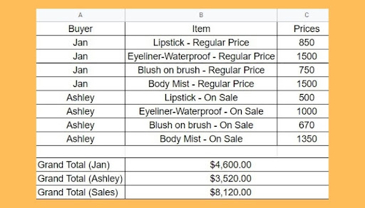
Mark is working as an auditor in one of the busiest innovative malls in the City. Mark’s boss, Kyle, wants him to extract the purchases of his girlfriends, Jan and Ashley, and consolidate it. He wants to make sure that what was on his list corresponds to the Pivot Table.
Mark uses the GETPIVOTDATA function to filter and extract the data from the Pivot Table easily. In just a second, Mark pulls up the following results:
Wondering how he did it? I’ll teach you how, but first let’s learn the basics.
The Anatomy of the GETPIVOTDATA Function
So the syntax (the way we write) the GETPIVOTDATA function is as follows:
=GETPIVOTDATA(VALUE_NAME,ANY_PIVOT_TABLE_CELL, [ORIGINAL_COLUMN, PIVOT_ITEM, ...])
- = every function in the Google Sheet always starts with an equal sign.
- GETPIVOTDATA() This function is used to extract the aggregated data from a Google Sheet Pivot Table report.
- VALUE_NAME is the name of the reference cell where you want to extract the data.
- ANY_PIVOT_TABLE_CELL refers to any reference cell in the pivot table. For this argument, it is advisable to use the topmost right cell of the pivot table.
- ORIGINAL_COLUMN This is an optional argument that refers to a source data set column. The column is not part of the pivot table report.
- PIVOT_ITEM refers to the name of the pivot table’s row or column that corresponds to the ORIGINAL_COLUMN that you want to extract.
A Real Example of Using GETPIVOTDATA Function
Here’s an example of how the GETPIVOTDATA function works in Google Sheets.
But first, you need to have a Pivot Table report as a source. If you have none, let us create one in the Google Sheet spreadsheet.
Here is the data that we will use to create the Pivot Table report.

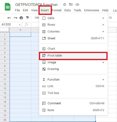
To make a Pivot Table, we need to go to the Insert menu and click on Pivot Table. However, in some instances, Google Sheets will not show the Pivot Table under the Insert menu.
What you can do is click on the ‘Help‘ menu on the toolbar. After clicking the Help menu, a search bar will pop up. Type in ‘Pivot Table‘ in the search bar.
Here’s what it looks like:

Once the Pivot Table menu is up, select the range you want to add to the Pivot Table.

Click on Insert, then click on Pivot Table.

The next step will look like this:

The Data Range is the range of the cells that you want to convert to a pivot table.
If you want to create a different sheet for your Pivot Table, you can click on the new sheet. Otherwise, select the existing sheet.
Here’s how it looks after applying the Pivot Table function. You must click ‘Add‘ to add the selected values from your source sheet.

For a detailed how-to guide on creating a Pivot Table, you may check this article.
Here’s the final out of our Pivot Table.

Let us now put it into practice. Before we proceed, you may click the link below to use the sample spreadsheet as you follow the guide.
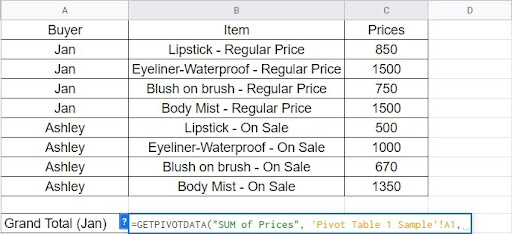
Now we will extract the grand total from each buyer and the total sales from this Pivot Table to our source sheet, Sheet1 Sample.
To extract the data from the Pivot Table, we will use this formula:
=GETPIVOTDATA(value_name, any_pivot_table_cell, [original_column, ...], [pivot_item, ...])
How to Use GETPIVOTDATA Function in Google Sheets
- First, substitute the source formula with the given data using this syntax:
The formula will now look like any of the formulas below.
Grand Total (Sales):
Grand Total Sales (from Buyer Jan):
2. In the source sheet, input the formula on the specified cell. Always start your formula with an ‘=‘ sign before the function.

3. After putting the function, add the field name of the cell which you want to extract the data from. Always add a comma after the field name.

Note: The field name should be enclosed with a ‘”‘ sign.
4. We will now add the Sheet name and the range cell of the Pivot Table which we will extract the data from.
5. Add the specific cell name and the specific value name or data that you want to extract.
Here, we will extract the total sales from the Buyer named Jan.
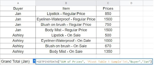
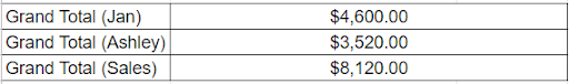
6. Here’s Buyer Jan’s Grand Total:
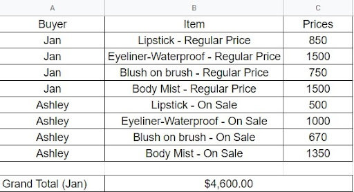
7. Cross-check the data with the Pivot Table’s data.

That’s it! It’s just that simple. Now, for your practice activity, find the return value of Buyer Ashley’s Grand Total.
Frequently Asked Questions
Why do I get an error on GETPIVOTDATA Function in Google Sheets?
There are various reasons why you get error messages when performing the GETPIVOTDATA function. But the most common causes why you are getting an #ERROR! error messages are as follows:
- The syntax – If the formula is not written correctly, it will yield an #ERROR! or #REF! error message.
- The Pivot Table – If the Pivot table’s range decreases, it will display the #ERROR! error message. This is why you should start the range with the topmost cell to cover the whole sheet. So when the Pivot Table’s size decreases, the
GETPIVOTDATAfunction will still work.
That’s it for today’s Google Sheet how-to guide. Start using them now! Don’t forget to sign up for our newsletter for more Google Sheet spreadsheet how-to articles like this.