How to use INDEX and MATCH Function with Multiple Criteria in Google Sheets

The INDEX and MATCH Function with Multiple Criteria in Google Sheets is useful if you want to look up a value with multiple criteria in a given table.

Meaning, the INDEX and MATCH function can also be used in looking up matches on more than one column at the same time.

The rules for using the INDEX and MATCH function with Multiple Criteria in Google Sheets are as follows:

• The function will return a #N/A error if no match is found based on the given criteria.
• The function can be set to have as many criteria as you want.
• 1 will be used as a constant value for search_key
• 0 or exact match will be used as a constant value for search_type.
• If there are multiple matches with the given conditions or criteria, the INDEX and MATCH function will return the first instance of the match.

Let’s take an example.

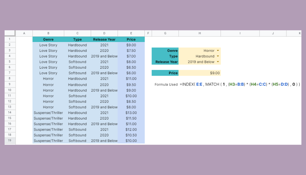
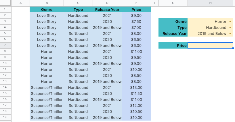
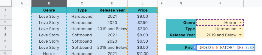
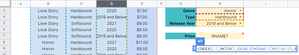
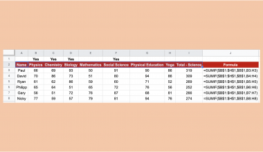
Jacob is working in a small retail bookstore. He’s trying to create a table in Google Sheets wherein after he picked the genre, type, and classification of a certain book his customer is buying, the price would automatically populate. See his table below:

With the knowledge of using the INDEX and MATCH function he learned from the Sheetaki website, he was able to successfully create a powerful tool that makes his job easier. Please see below:

The price field in cell H7 automatically populates based on the table on the left side. All Jacob has to do is supply the data in cells H3, H4, and H5 according to the customer’s preference. After that, the price of the book will be pulled and shown in cell H7.

Pretty amazing, isn’t it?

Watch out for a more advanced tutorial and examples on how you can use the INDEX and MATCH function with multiple criteria in the coming weeks. Be sure to subscribe to be notified. 

Awesome! Let’s begin getting to know more about our INDEX and MATCH function with multiple criteria in Google Sheets.

The Anatomy of the INDEX and MATCH Function used with Multiple Criteria

So the syntax (the way we write) the INDEX and MATCH function is as follows:

=INDEX(reference,MATCH(1,(criteria1)*(criteria2)*(criteria3)*...(criteria_N),0))

Let’s dissect this thing and understand what each of these terms means:

• = the equal sign is just how we start any function in Google Sheets. It is how Google Sheets understand that we are asking it to either do computation or use a function.
• INDEX() function retrieves a value from a specific range.
• reference is the range where you want to get your data.
• MATCH() function gives the position of your search key defined by the criteria.
• 1 is our fixed search key or the value that we are looking for.
• criteria1, criteria2, criteria3…criteria_N criteria or the conditions you are looking to match.
• 0 is our fixed search type, which controls that we’re searching for an exact value.

Please visit this INDEX and MATCH function article for more in-depth explanations and examples.

A Real Example of Using INDEX and MATCH Function with Multiple Criteria

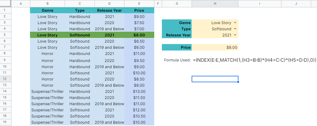
Take a look at the powerful tool that Jacob created to see how the INDEX and MATCH function with multiple criteria is used in Google Sheets.

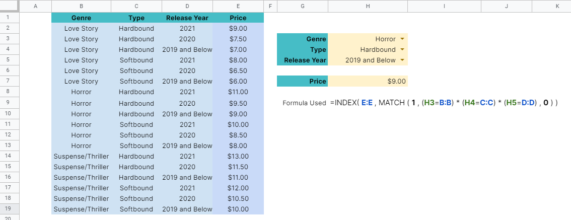
The value in cell H7 was obtained using the following syntax:

=INDEX(E:E,MATCH(1,(H3=B:B)*(H4=C:C)*(H5=D:D),0))

Notice that there are two functions used in the above formula, the INDEX and MATCH functions. The MATCH function is nested inside the INDEX function. 

The role of the INDEX function above is to retrieve a value from a specific range defined in its first argument. In this case, column E or simply E:E. This means that we want the entire formula to return a value from column E.

It can be any of the columns from B to E. However, in the example above, the goal is to return the price of a certain book based on customer preferences. Hence, column E is used.

The role of the MATCH function is to tell the position of what we are looking for, in this case, we are looking for the value 1. This is the first and fixed argument in our MATCH function whenever we are using multiple criteria in the INDEX and MATCH functions.

The second argument of our MATCH function is the list of criteria or conditions that we are looking for in our provided cell range or table.

(H3=B:B) * (H4=C:C) * (H5=D:D)

In our example, there are three conditions that we set. These conditions are based on the customer’s book preference. The Genre (H3), Type (H4), and Release Year (H5). 

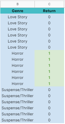
Let’s take a look at our first condition:

H3=B:B

This means that we are trying to check if there will be a match of what’s in H3 in column B. If there is a match, it would return the TRUE value or 1. Otherwise, it would give the FALSE value or 0. 

In our example, since the value in H3 is ‘Horror’, there should be 5 matches in column B:

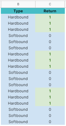
Our second condition or criteria is defined by the below formula:

H4=C:C

Similar to our first condition, this means that we are trying to check if there will be a match of what’s in H4 in column C. The return value should be either TRUE/1 or FALSE/0.

Since the value in H4 is ‘Hardbound’, there are 9 matches in column C:

As for our last condition, we defined it using the following formula:

H5=D:D

We are trying to check if there’s a match of what’s in H5 in column D. In our example, we are looking for the text ‘2019 and Below’. There are 6 matches in our cell range:

This is where it gets exciting. Notice the operations between each condition. The asterisks(*) between each condition denote multiplication. 

This means that for the list of conditions that we set, we are only returning two possible values, either 1 or 0. Please see below:

Remember that we passed the value 1 as the first argument of our MATCH function? This means that we are looking for the resulting exact match, defined by 0 as the third argument of our MATCH function.

Our MATCH function will see the results above and will return the position of 1. 

This then will be passed to the INDEX function, which will be treated as its second argument.

The INDEX function will return the corresponding value in the cell range or our table based on the position provided by the MATCH function. 

In this case, since we asked to return the value in column E, it yielded the value of $9.00.

You may make a copy of the spreadsheet using the link I have attached below.

How to Use INDEX and MATCH Function with Multiple Criteria in Google Sheets

1. Click on any cell to make it the active cell. For this guide, I will be selecting H7, where I want to show my result.

2. Next, type the equal sign ‘=‘ to begin the function and then follow it with the name of the function, which is our ‘index‘ (or ‘INDEX‘, not case sensitive like our other functions).

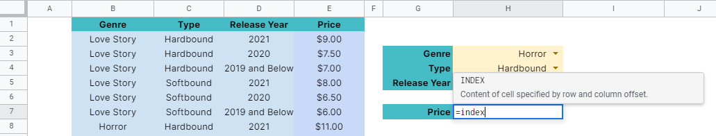
3. Type open parenthesis ‘(‘ or simply hit Tab key to let you use that function.

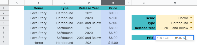
4. Now the exciting part! Let’s give our function its first argument, the reference. Click the column E, or manually type in E:E.

5. To let the Google sheet know that we’re done typing our first argument, we should now type in the delimiter or the character that separates each argument on a function. In this case, type comma ‘,’.

6. Type in our second argument, which is the MATCH function. Type in ‘match’ or ‘MATCH’ (not case sensitive) then hit the TAB key.

7. Pass to the MATCH function its first argument, which is the value 1, and follow it with the delimiter.

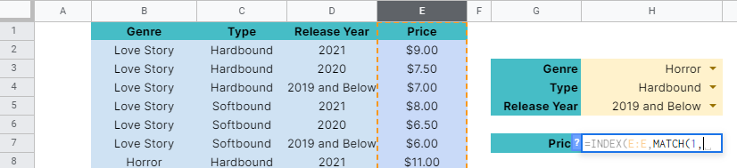
8. Now, provide the conditions enclosed with the open and close parenthesis “()“. These conditions should be separated by the asterisk(*).

9. Type in the first condition, which is ‘(H3=B:B)’. You can type it directly as it is or you can type open parenthesis ‘(‘, then click the cell H3. Follow it with the equal sign (=) then column B.

10. We are done typing the first condition. Now, type in asterisk (*) and follow it with the second condition. In this case, type in ‘(H4=C:C)’. Alternatively, you can type it the same way you typed in the first condition.

11. Type another asterisk (*) and follow it with the third condition. Type in ‘(H5=D:D)’.

12. Since we only have 3 conditions, let’s proceed with the comma (,) as the delimiter, and follow it with the third argument of the MATCH function, which is 0.

13. Finally, hit your Enter or Tab key. Cell H7 will now show you the result or the return value of the INDEX and MATCH function.

14. You may try a few tests with our formula by changing the values in H3, H4, and H5.

That’s pretty much it. You can now use the INDEX and MATCH function with Multiple Criteria in Google Sheets together with the other numerous Google Sheets formulas to create even more powerful formulas that can make your life much easier.

Get emails from us about Google Sheets.

Our goal this year is to create lots of rich, bite-sized tutorials for Google Sheets users like you. If you liked this one, you'll love what we are working on! Readers receive ✨ early access ✨ to new content.

Subscribe