This guide will explain how to use the ISERR function in Google Sheets.
When we need to check whether a value is an error other than #N/A, we can easily do this using the ISERR function in Google Sheets.
Table of Contents
The rules for using the ISERR function in Google Sheets are the following:
- The
ISERRfunction considers all error types as errors except for the #N/A error. - The
ISERRfunction will return FALSE on #N/A errors since it does not treat it as an error. Otherwise, the function will return TRUE on the rest of the errors such as #VALUE!, #NAME? or #NUM!. - The
ISERRfunction is best used with other functions for efficiency, such as theIFfunction in conditional statements.
Google Sheets has several built-in functions that let us accurately perform complex tasks. Despite this, errors can happen when performing calculations and other tasks.
There are many types of error-checking functions in Google Sheets. For example, there are the ISERROR function, the ISNA function, and the ISERR function.
We will focus on the ISERR function, which is used to check whether a value is an error except for a #N/A error. An #N/A error means that no value is available or the formula cannot find what it is asked to look for.
In this guide, we will provide a step-by-step tutorial on how to use the ISERR function in Google Sheets. We will explore the syntax and a real example of using the function.
Great! Let’s dive right in.
The Anatomy of the ISERR Function
The syntax or the way we write the ISERR function is as follows:
=ISERR(value)
- = the equal sign is how we begin any function in Google Sheets.
- ISERR() is our
ISERRfunction. This function is used to check whether a given value is an error other than the #N/A error. - value is the only required argument. This refers to the value we want to verify as an error type other than the #N/A error.
The Anatomy of the IF Function
The syntax or the way we write the IF function is as follows:
=IF(logical_expression,value_if_true,value_if_false)
- = the equal sign is how we activate any function in Google Sheets.
- IF() refers to our
IFfunction. This function is used to return one value if a logical expression is TRUE and another value if it is FALSE. - logical_expression is a required argument. This refers to an expression or cell reference containing an expression that represents some logical value i.e. TRUE or FALSE.
- value_if_true is another required argument. This refers to the value we want the function to return if logical_expression is TRUE.
- value_if_false is also a required argument. This refers to the value we want the function to return if logical_expression is FALSE.
Note: Make sure to provide the value_if_true and value_if_false arguments in the correct order–this is the single most common error made when using the IF function.
Types of Error-Checking Functions in Google Sheets
There are many ways to handle errors in Google Sheets using different functions. Moreover, each error-checking function is used for specific situations.
Firstly, the ISERROR function checks whether a value is an error. This is best used to identify any type of error in our data set.
Secondly, the ISNA function checks whether a value is the error #N/A error. The ISNA function will only return TRUE if the given value is a #N/A error. Otherwise, the function will return FALSE.
Lastly, the ISERR function is opposite to the ISNA function. The ISERR function checks whether a value is an error except for the #N/A error.
Thus, the ISERR function will return TRUE for all types of errors unless it is a #N/A error. Then, the function will return FALSE.
It is important to learn the difference between error-checking functions to be able to use the most appropriate function for the data set.
A Real Example of Using ISERR Function in Google Sheets
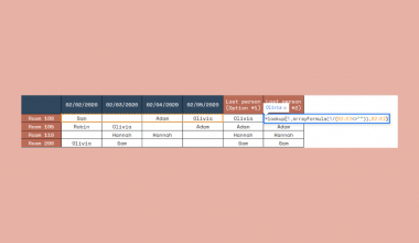
Let’s say we have a data set containing a few errors. We want to handle all the errors except for the #N/A errors. Our initial data set would look like this:

In the spreadsheet above, we can see all kinds of errors. Let’s say we want to check all the values to see whether it is an error. But we want to exclude the #N/A errors.
We can easily do this using the ISERR function:
=ISERR(C2)

The formula above only has one argument. We simply selected the cell C2 which contains the value we want to check for errors.
The ISERR function will return TRUE for all errors except for the #N/A error. Hence, the cell containing the #N/A error returned FALSE.
Since we have verified the errors in our data set, we now want to return a custom value when an error is detected. We do this by using the ISERR function together with the IF function.
For example, we want to return “error detected” when the function finds an error and “no error” for the #N/A error.
We can perform this task using the formula:
=IF(ISERR(C2),"error detected","no error")

The first part of the formula is our logical_expression argument. In this case, we inputted our ISERR formula. Then, we specified what value we want to return if the logical_expression is TRUE which is “error detected”.
Since our logical_expression is the ISERR formula, it will only return TRUE if an error except for #N/A is detected. Lastly, we will input “no error” as the value_if_false argument.
Our final data set would look like this:

You can make your own copy of the spreadsheet above using the link below.
Amazing! Now we can dive into the steps of using the ISERR function in Google Sheets.
How to Use ISERR Function in Google Sheets
1. First, we will create a new column in the data set to display the results from the ISERR function.

2. We will start our formula by typing an equal sign and the function name. The formula would become “=ISERR(”.

3. Then, we will simply select the cell containing the value we want to check for errors. The formula would become “=ISERR(C2) ”.

4. We will press the Enter key to return the result.

5. Next, we will drag down the Fill Handle tool to apply the formula to the other cells.

6. Now that we have verified the errors, we want to return a specific value when an error is found except for #N/A. To begin our formula, we will input an equal sign and the function name. The formula would become “=IF(”.

7. We will input our ISERR formula as our logical_expression argument. Then, the formula would be “=IF(ISERR(C2),”.

8. We want the function to return “error detected” when the ISERR formula returns TRUE. In this case, the formula would become “=IF(ISERR(C2),”error detected””

9. Next, we will type “no error” when the ISERR formula returns FALSE. The final formula would become “=IF(ISERR(C2),”error detected”,”no error”)”.

10. We will press the Enter key to return the result.

11. Lastly, we will drag down the Fill Handle tool to copy the formula to the rest of the column.

And tada! We have successfully used the ISERR function in Google Sheets.
You can apply this guide whenever you need to check whether a value is an error except for the #N/A error. You can now use the ISERR function and the various other Google Sheets formulas available to create great worksheets that work for you.
That’s pretty much it! Make sure to subscribe to our newsletter to be the first to know about the latest guides and tutorials from us.