This guide will explain how to paste a range of values in reverse order in Excel.
We’ll provide two different methods you can use to copy and paste a range of values in reverse order.
Suppose you have a sign-up sheet for an event written in Excel. The latest entries are found lower in the worksheet.
We want to copy all the contact details from the sheet and paste it elsewhere. We must also to present these details in reverse. For example, the contact details of the last person who signed up to appear first on our new list.
How can we do this in Excel easily?
We will provide two ways to reverse the order of a range in Excel.
First, we’ll show you how to reverse a list using Excel formulas. The advantage of using this method is that it updates automatically whenever the original list is edited.
Next, we’ll show how you can use Excel’s Sort command to reverse the order of a list. This method is simpler to implement but requires setting up a helper column.
The use case above is just one of many possible scenarios that require you to reverse a list. The methods in this guide will also be useful if you’re having difficulty sorting data that does not have a timestamp.
Now that we have a grasp on when to reverse the order of a range of values, let’s learn how to use it on an actual sample spreadsheet.
A Real Example of Pasting Values in Reverse Order in Excel
The following section provides several examples of how to paste values in reverse order. We will also go into detail about the formulas and tools used in these examples.
In the example below, we have a list of first names in no particular order. If we want to sort this list, we must provide an explicit value of the position of each name in the range.
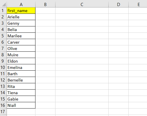
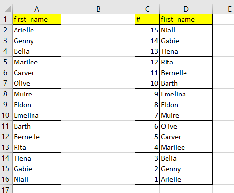
We can add a helper column that indicates the position of each name in the list. For example, column C tells us that Arielle is the first name in the list and that Tiena is the 13th.

We can now sort column C in reverse order. Excel will automatically sort the adjacent column D through the ‘Expand the Selection’ feature.
We can also use the OFFSET function to output the last value in the range.
=OFFSET($B$10,-(ROW(B2)-2),0)
When the user uses the Fill Handle tool to copy the formula above, the output ROW function will increment by 1. This allows the OFFSET function to return the second-to-the-last value and so on.
Do you want to take a closer look at our examples? You can make your own copy of the spreadsheet above using the link attached below.
If you’re ready to try out pasting the values in reverse order in Excel, head over to the next section to read our step-by-step breakdown on how to do it!
How to Paste in Reverse Order in Excel
This section will guide you through each step needed to reverse the order of a range of values in Excel. You’ll learn how we can use the Sort feature and the OFFSET function to achieve this.
Follow these steps to paste your results in reverse order in Excel:
- Let’s start with the method that uses Excel functions. First, select the cell where you want to place your reversed copy. In this example, we’ve selected cell C1.

- Paste the
OFFSETfunction into the formula bar. Ensure that the first argument is an absolute reference to the last cell in the range. TheROWfunction’s argument should be the first cell in the range.

- Hit the Enter key to evaluate the function. In our example, the
OFFSETformula returned ‘Niall’, the last value of the range in column A.

- Use the Fill Handle tool to make a copy of the formula in cell C1. The new range should show the original values in reverse order.
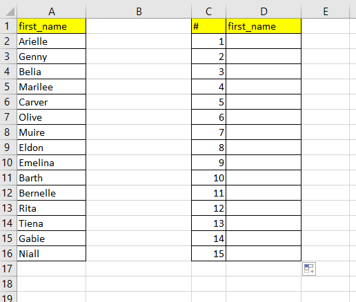
- Next, we’ll try to use Excel’s Sort feature to reverse the order of a range. First, we’ll create a helper column with a range of numbers from 1 to the length of your range. In this example, we’ve added a range of numbers from 1 to 15 in column C.
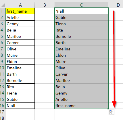
- Copy and paste the original values into a column adjacent to the helper column.
- Select both the helper column and the duplicated list of values. In this example, we’ve selected the range C1:C16.

- Right-click on the selection and click on the option Sort Largest to Smallest.
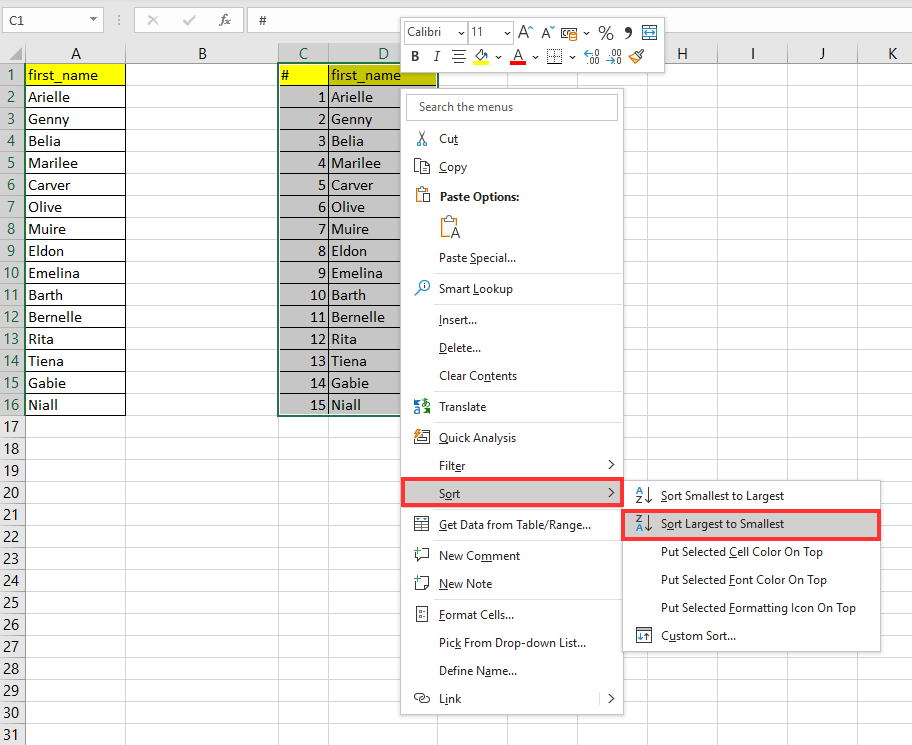
- The copy you’ve made should now be in reverse order.
These are all the steps needed to reverse the order of copied cells.
This step-by-step guide should provide you with all the information you need to paste a range of values in reverse order. We’ve shown two ways you can perform this operation in Excel: using the Sort feature and using the OFFSET function.
This function is just one example of the many Excel functions that you can use in your spreadsheets. Our website offers hundreds of other functions and methods to help you get more out of Microsoft Excel.
With so many other Excel functions available, you can find one appropriate for your use case.
Subscribe to our newsletter to look into the latest Excel guides and tutorials from us.