


This guide will explain how to use the PERCENTIF function in Google Sheets.
This means you can get the percentage of a range that meets a specific condition you have set in Google Sheets using the PERCENTIF function. So you can apply this function to quickly identify when a value in your dataset meets the specific condition you have set.
The rules for using PERCENTIF in Google Sheets are as follows:
- If the range to be checked against contains a text, the criterion must be a string.
- If the range to be checked against contains numbers, the criterion can be either a string or a number.
- The criterion must be enclosed in quotation marks.
- It can only support a single criterion.
Let’s take an example.
Suppose you are a sales team manager. For this reason, you want to monitor the percentage of employees in your team that is performing well or underperforming.
But it would be difficult to check each employee’s weekly performance and calculate its percentage when it increases or decreases. And not to mention it would take up so much time. Hence, you make use of the PERCENTIF function to monitor their performance.
Great! That’s just one example out of many of using the PERCENTIF function in Google Sheets. Besides the PERCENTIF function is very helpful in similar situations or when dealing with percentages.
Since we have dealt with one example, let’s discuss how you write and use the PERCENTIF function on your Google Sheets.
The Anatomy of the PERCENTIF Function
So the syntax (the way we write) of the PERCENTIF function is as follows:
=PERCENTIF(range, criterion)
Let’s dissect the parts of this function and understand what each term means:
- = the equal sign is just how we start any function in Google Sheets.
- PERCENTIF() this is our
PERCENTIFfunction.PERCENTIFreturns the percentage of a range that meets a specific set condition. So it will take the selected range to check against the specific criteria you have set and give the percentage based on that. - range is the selected cells that will be tested against the criterion. Also, these can be numbers, currencies, or even names.
- criterion is the criteria or condition you have set to apply to the range. And this can be a text, numbers, or even wildcards such as a question mark. Also, it can be a number prefixed with the following operators: =, <, >, <=, or >=, which check if the range is equal to, less than, greater than, less than, or equal to, or greater than or equal to the criterion, respectively. Additionally, the criterion must be enclosed in quotation marks.
Note: The PERCENTIF function automatically formats the results as percentages.
A Real Example of Using PERCENTIF Function in Google Sheets
First, let’s look at the example below to see how the PERCENTIF function is used in Google Sheets. This is the spreadsheet that you will be using:
So you are a teacher keeping records of a class. First, you want to monitor the percentage of students who passed and failed the test. Furthermore, you keep a record of the number of males and females in the class. To calculate all of this easier, you make use of the PERCENTIF function.
As you can see, the PERCENTIF function gives a percentage result based on the range you selected and the criterion you set.
You may make a copy of the spreadsheet using the link I have attached below.
How to Use PERCENTIF Function in Google Sheets
In this section, you will learn how to use the PERCENTIF function step-by-step. Each step will contain detailed instructions and images to guide you throughout the process.
1. First, type the ‘=’ to start the function.
2. Second, type the name of the function, ‘PERCENTIF’. As you are typing, a dropdown menu will appear. From there, you can click PERCENTIF.
3. Next, select the range you will be testing, which is the score column. After, enter the criterion. For example, you want to find the percentage of students who passed the test, or in this case, who scored equal to or greater than 35.
For the criterion, type in ‘>=35’. Your entire syntax will be =PERCENTIF(C2:C11,”>35”). Lastly, press enter to show the result. Also, the criterion must be enclosed in quotation marks. If not, it will result in a #ERROR! 
4. Then, you want to find the percentage of students who failed the test. Then, you can follow the same steps. But this time, your criterion will be less than 35. Type in ‘<35’. Your entire syntax should be =PERCENTIF(C2:C11,”<35”). And press Enter to show the result.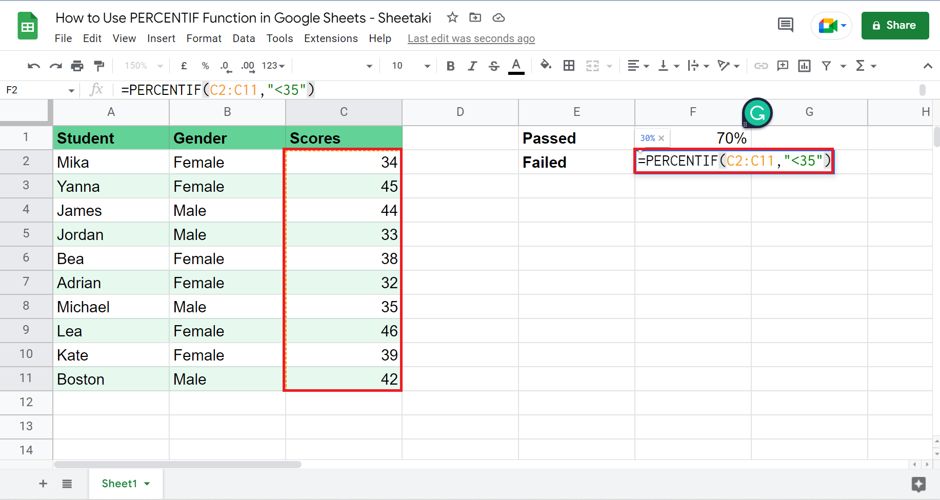
5. Let’s try using text for the criterion. For instance, you want to find the percentage of females in the class. It follows the same process, but with a different criterion.
After selecting the range, which in this case is the gender column, you can type in the criterion ‘Female’. Don’t forget the quotation marks. For this case, the syntax should be =PERCENTIF(B2:B11,”Female”). Lastly, press Enter.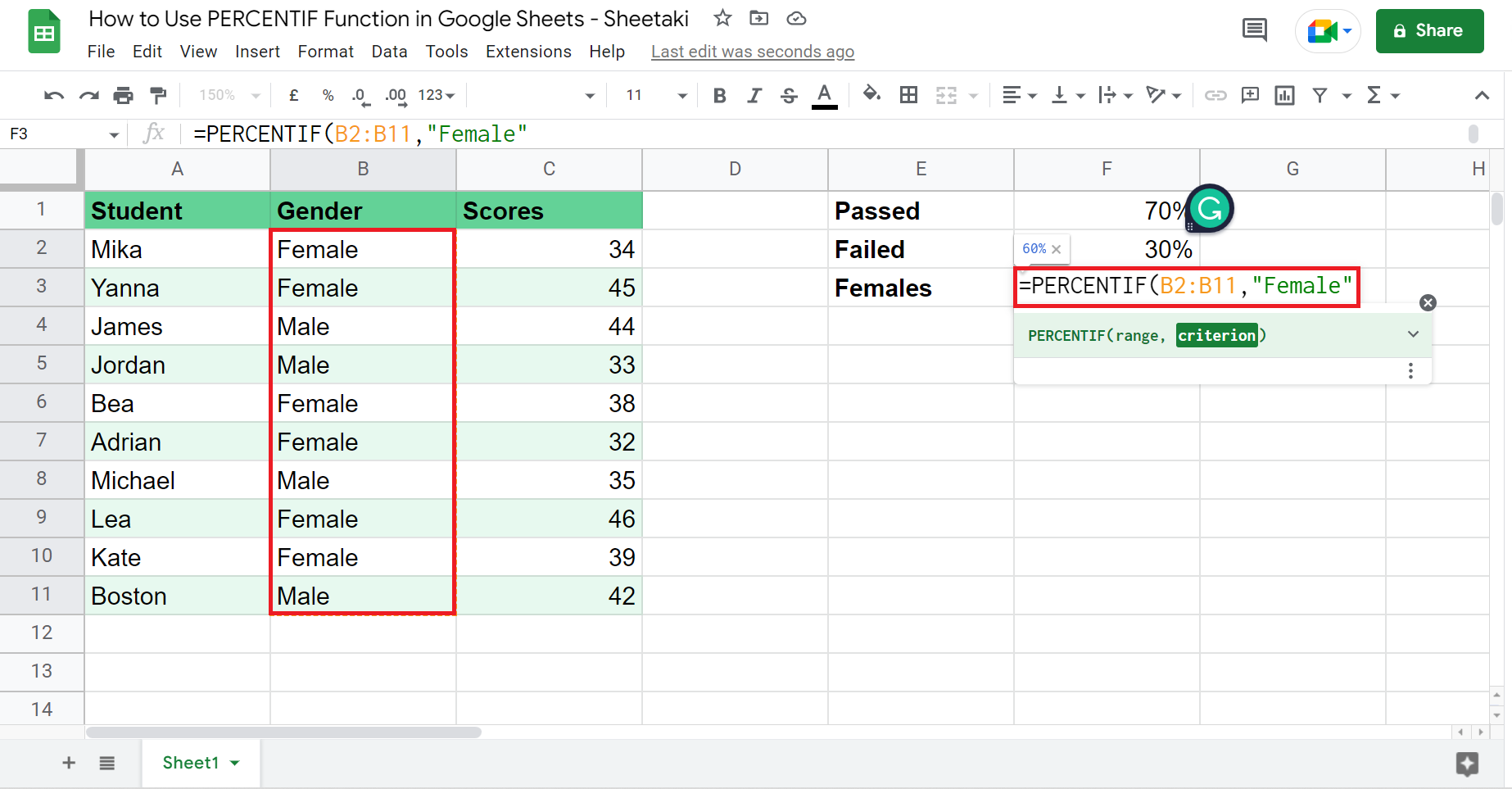
6. Next, let’s look at the percentage of males in the class. First, type in the ‘=’ to start the function. Select PERCENTIF and the range, which is still the gender column.
Then, type in ‘Male’ for the criterion. The syntax for this should be =PERCENTIF(B2:B11,”Male”). Finally, press Enter to show the results. 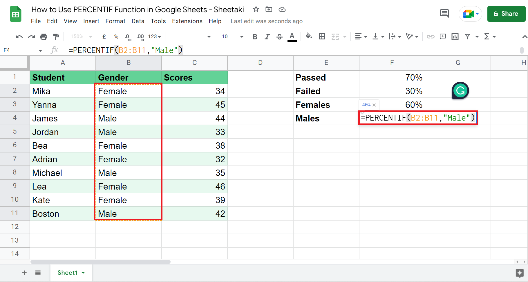
7. Lastly, let’s try using a wildcard for the criterion. For instance, you want to know the percentage of students with a name that starts with J. First, follow the same process as before.
Only the criterion part is different. After selecting the range, which in this case is the student column. Then, type ‘J*’ for the criterion. The syntax should look like this: =PERCENTIF(A2:A11,”J*”). And press Enter to show results.
8. And tada! Finally, this is what it would look like after using the PERCENTIF function.
That’s pretty much it. So you can now use the PERCENTIF function with different criteria. May they be a number, a text, or even a wildcard. Also, you can apply this to your work to make it more efficient and easier for you when dealing with percentages.
The T.DIST function is just one example of a statistical function you may use in Google Sheets. With so many other Google Sheets functions out there, you can surely find one that suits your data.
Are you interested in learning more about what Google Sheets can do? Make sure to subscribe to our newsletter to be the first to know about the latest guides and tutorials from us.


