This guide will discuss how to do product codes in Excel using the data validation tool.
Excel is an excellent tool with many tools and features for many tasks, such as reports, calculations, and data analysis. And one more thing Excel is an excellent tool for is keeping product inventory.
Because Excel has many functions and tools that make it easy to store and input data, people often use Excel to create an inventory of their products. And this product inventory can contain necessary information.
For instance, the product inventory can contain the product name, quantity, and product code. So a product code is an important unique series of numbers attached to a product in order to keep track of it.
But, the question is, how do we do product codes in Excel? Worry not, this guide will discuss how to do product codes in Excel.
Let’s take a sample scenario.
Suppose you were tasked to create an inventory of your company’s products in Excel. So you wanted to find out how to do product codes in Excel easily and quickly in order to finish your task efficiently. Additionally, this would save time, especially when dealing with a large inventory of products.
Awesome! Now let’s move on and dive into a real example of how to do product codes in Excel.
A Real Example of Doing Product Codes Excel
Let’s say we were asked to create a product inventory containing the product name, the quantity of the product, and the product code.
So we will be utilizing the data validation feature. Firstly, we will be applying data validation so that we can only show the product code when selecting an item. And to do that, we will create a dropdown list menu containing the product name and code.
Then, we will prepare the other needed aspects, such as turning the data set into a table and a named range. Next, we will create the dropdown list using data validation.
Afterward, we would have attached a dropdown list to our data set. So we can now easily select the product codes. And our final output would look something like this:

You can make your own copy of the spreadsheet above using the link attached below.
Great! Now we can dive into learning about the step-by-step process of how to do product codes in Excel using data validation.
How to Do Product Codes in Excel
In this section, we will discuss the step-by-step process of how to do product codes in Excel using the data validation feature. Furthermore, each step will contain pictures and detailed instructions to guide you along the process.
1. Firstly, we need to prepare our codes. So the codes will contain the product number, the product name, and the product show, which is the combination of the product name and code. To create a product show, type in the formula “=B3&”–”A3”. Then, press the Enter key to return the results.

2. After, copy down the formula by dragging it down to the rest of the column.

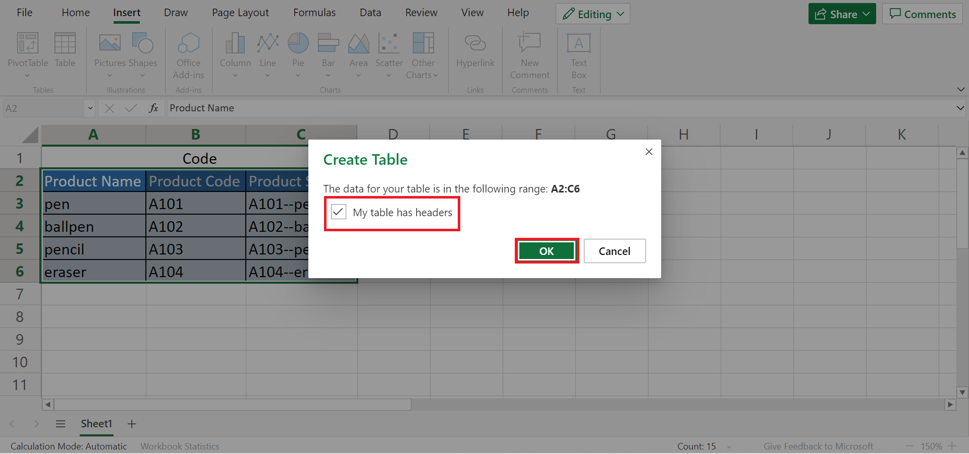
3. Secondly, we will create an Excel table. So we will select the data set. Then, go to the Insert tab and click Table.

4. Next, check the box for My table has headers. Lastly, click OK to apply the changes.

5. Then, let’s sort the list by the product name to make it easier to find the products in the dropdown list. To do this, go to the Data tab and click Sort Ascending.

6. Next, we need to create a named range beside the product show column. Firstly, we need to click at the top of the product show column to select the data, excluding the header. Then, go to the Formulas tab. And select Define Name and enter a name for the range.

7. So, in this case, we will name it “ProductList”. Lastly, click OK to add the name.

8. Afterward, we can finally add the dropdown list. So select all the cells where the dropdown list is needed. Then, go to the Data tab and select Data Validation.

9. When the Data Validation window appears, go to the Validation criteria and select List in the Allow dropdown menu. Next, input “=ProductList” under Source. Lastly, click OK to apply the data validation.

10. And tada! Now we have created a dropdown list showing the product show details of the product. Only the product code appears on the cell when selecting an item from the dropdown list. So we have successfully done product codes in Excel.

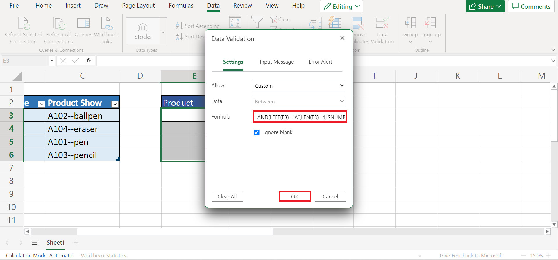
11. We can also use data validation to prevent customers or other people from inputting incorrect product codes. Firstly, select the Product column. Then, go to the Data tab and select Data Validation.

12. And the Data Validation window will open. Next, select Custom in the Allow dropdown menu. Then input the formula “=AND(LEFT(E3)=”A”,LEN(E3)=4,ISNUMBER(VALUE(RIGHT(E3,3))))”.
Essentially, the custom formula is making sure the inputted product code starts with the letter A, has a length of four characters, and ends with three numbers. Finally, click OK to apply the data validation.

13. And tada! We have successfully added a data validation to prevent inputting incorrect product codes.

And that’s pretty much it! We have discussed how to do product codes in Excel using the data validation feature. Furthermore, we have explained how to add data validation to prevent incorrect product codes. And now, you can successfully do product codes in your own work whenever necessary.
Are you interested in learning more about what Excel can do? You can now use the various other Microsoft Excel formulas available to create great worksheets that work for you. Make sure to subscribe to our newsletter to be the first to know about the latest guides and tutorials from us.


