The PRODUCT function in Google Sheets is used to return the result of multiplying a series of numbers together.
Table of Contents
The PRODUCT function is a simple function that acts as a multiplication function in Google Sheets.
While you can use the usual asterisk or * sign, the PRODUCT function has other practical uses.
Let’s take an example.
As a catering service in our want to be able to find out how many meals you should prepare for school event happening in your city.
You need to know the total number of schools, classes per school, students per class, and meals per student you should prepare.
How should we go about that?
Fortunately, the PRODUCT function just needs an input value, which could be as many inputs as you like.
We will discuss the real examples and actual values to see how to use the PRODUCT function in Google Sheets.
The Anatomy of the PRODUCT Function
The syntax (the way we write) the PRODUCT function is simple:
=PRODUCT(factor1,[factor2,...])
Let’s break this down to understand the syntax of the PRODUCT function and each term:
=the equal sign is how we begin any function in Google Sheets.PRODUCTis our function. We need to add the factor attribute for it to work properly.factor1, [factor2,...]is the only attribute of this function. It is the cells that act as factors in our calculation.
The advantage that PRODUCT has over using the * or asterisk is that you can multiply over a range or a table in a quick and efficient manner, instead of inputting the values or cell addresses that you need to multiply one by one.
The advantage that PRODUCT has over using the MULTIPLY function is that MULTIPLY only works with two factors. In PRODUCT, it is listed that you can have up to 30 factors, but if you indeed need more, PRODUCT supports an arbitrary number of arguments.
Each factor can be a specified number or a range. If there are blanks within the specified range, they are ignored and won’t affect the end product.
A Real Example of Using PRODUCT Function
Let’s look at this example below to see how to use the PRODUCT function in Google Sheets.
Finding the Product of More Than 2 Factors in Google Sheets
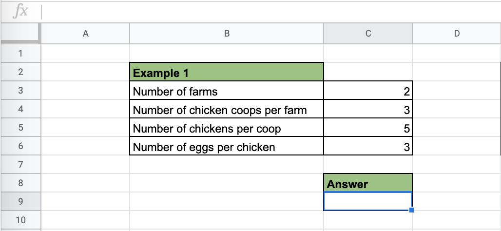
In this simple problem, we want to find out how many meals we need to make as caterers for some school parties.

The function with a cell reference is:
=PRODUCT(F3:F6)
As a result, we will get 600.
This simple problem can be practiced. Use the link below to use our spreadsheet sample:
How to Use PRODUCT Function in Google Sheets
In this section, we will show you a step-by-step process on how to use the PRODUCT function in Google Sheets.
Finding the Product of More Than 2 Factors in Google Sheets
- To begin, click on the cell where you want to show your result to make it the active cell. In this guide, we will choose C9, where I want to see the result of our calculation.
- Next, type the equal sign ‘=’ to start off the function. After that, followed by the name of the function which is ‘product’ (or PRODUCT, which also works).
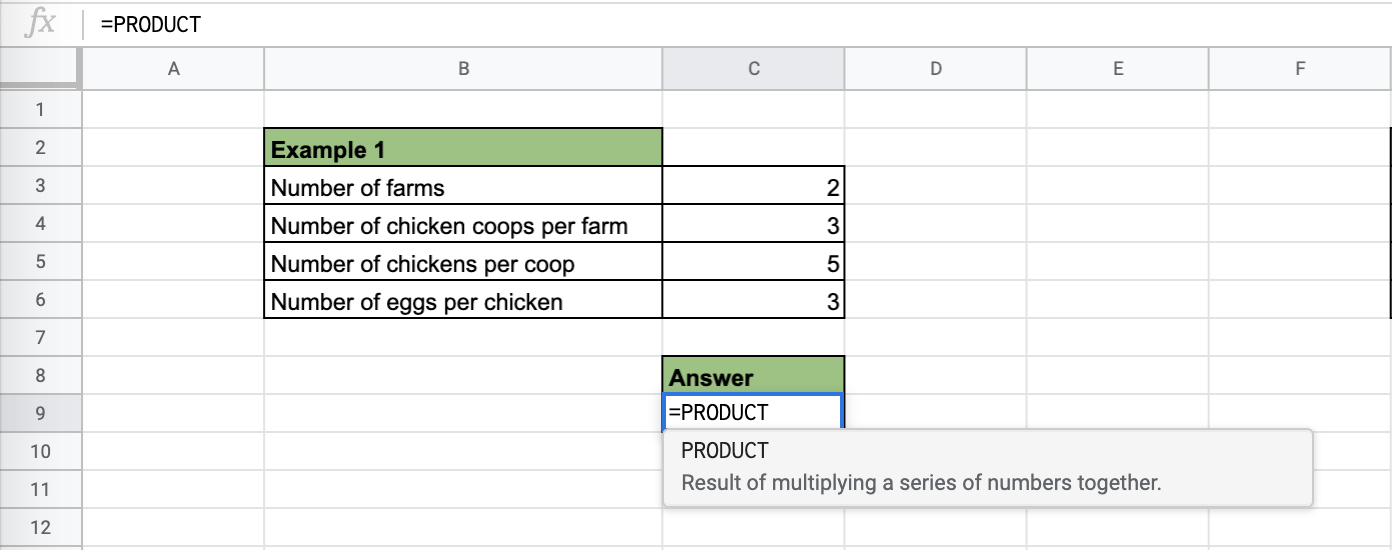
- You can now see the auto-suggest box will pop-up with the name of the functions that start with
PRODUCT. Select thePRODUCTfunction by clicking on it. Make sure to choose the correct function.
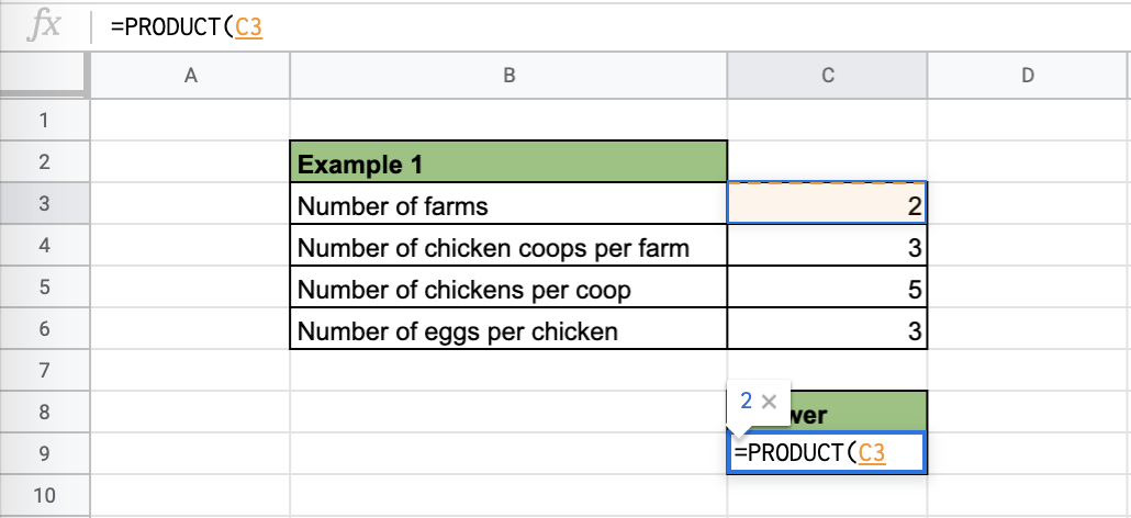
- After the opening bracket ‘(‘, you will have to add the factor1 attribute. Note that you can put in a range, or choose the cell addresses you want to add. Note that you also get a preview of the answer you need as you add factors or add to the range of numbers.

- You could also add the factors you need one-by-one if the numbers you need to multiple are not arranged in a column/row range.
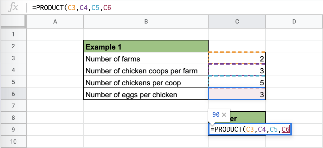
- Close the function with the closing bracket.
- Finally, hit the Enter key to close the whole formula and it will output the result. You should now have the proper number of your desired answer.

That’s it, you’re done! You can now use the PRODUCT function together with other Google Sheets formulas and create even more powerful and amazing formulas.