How to Use SUMIF with OR in Excel

This guide will explain how to use SUMIF with OR logic in Excel.

We can use the SUMIF function to total all values in a range that has a corresponding value in another field that fits our criteria.

The SUMIF function allows users to add up all cells in a range that fits a particular condition. For example, we might want to find the sum of all expenses made in January or the total profit coming from a particular product. 

However, we can also use the SUMIF function to add all cells that fit one of the multiple criteria. Let’s take a look at a quick example where you might need to add values in a range that fit one of several criteria.

Suppose you have a dataset of transactions made in 2022. You want to know the number of transactions coming from users based in either New York or Los Angeles. 

We can use the SUMIF function to calculate the number of people from both New York and Los Angeles. We can add the result of both of these formulas to find the total.

Excel also allows us to provide an array of conditions as an argument in our SUMIF function. We must use the SUM function to get the total of all the results.

Now that we know when to use the SUMIF function, let’s learn how to use it on an actual sample spreadsheet.

A Real Example of Using SUMIF with OR in Excel

The following section provides several examples of how to use the SUMIF function given multiple acceptable criteria. We will also explain the formulas and tools used in these examples.

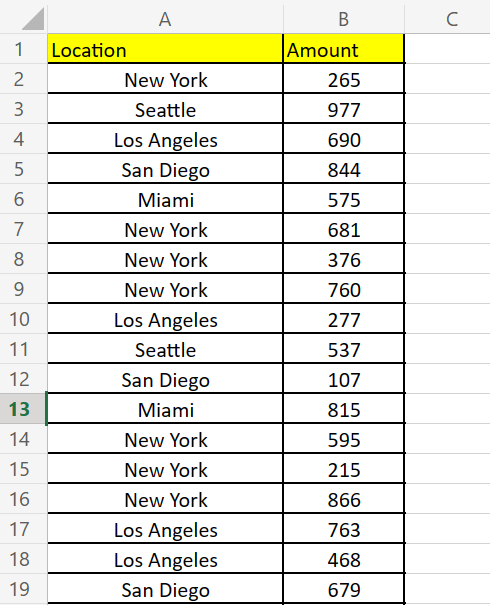
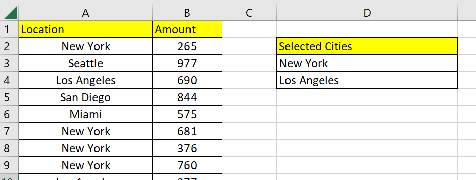
First, let’s take a look at our sample data. Our spreadsheet has a  list of transactions with a corresponding location and transaction amount. We want to return the total amount of all transactions coming from either New York or Los Angeles.

We can write down the list of acceptable locations in the same sheet to use in our formula.

To get the sum seen above, we just need to use the following formula:

=SUM(SUMIF(A2:A21;D3:D4;B2:B21))

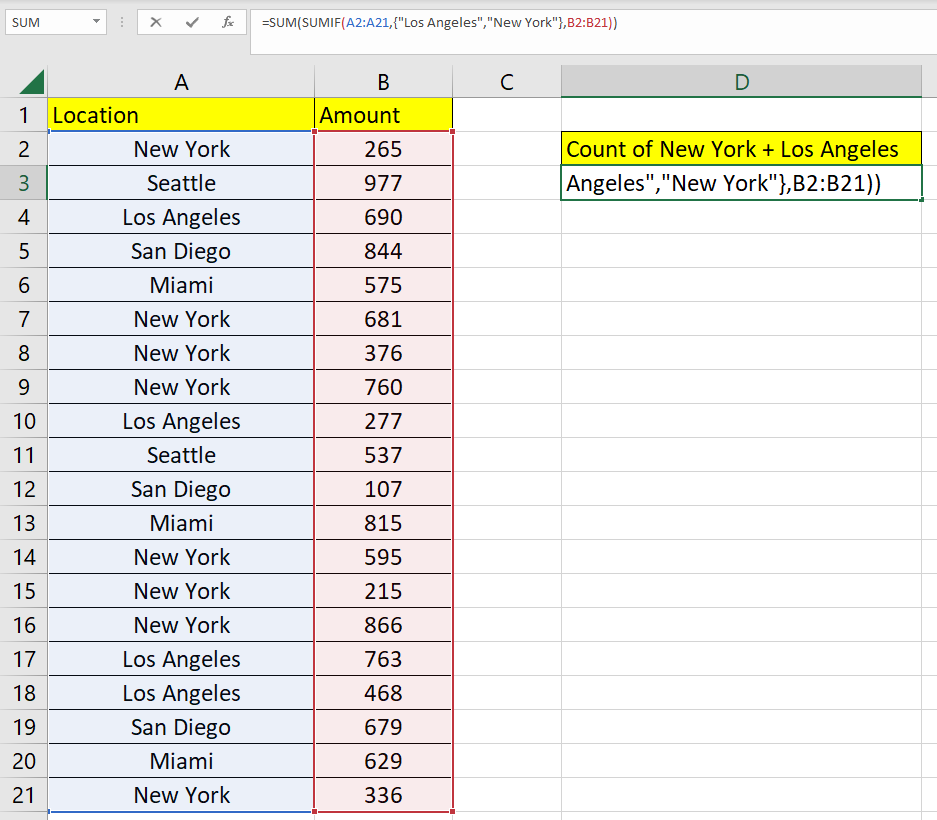
Instead of using a cell reference, we may also use an array of acceptable strings as an argument:

=SUM(SUMIF(A2:A21;{"Los Angeles","New York"};B2:B21))

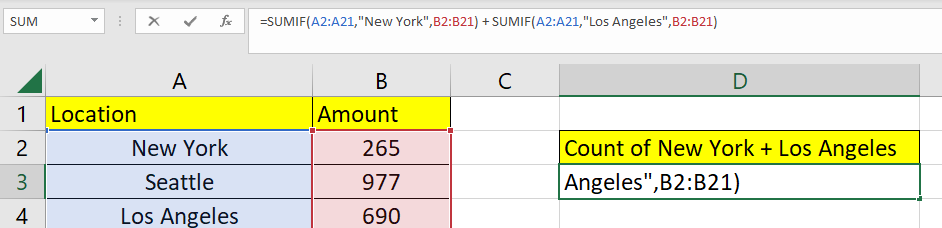
Another alternative to adding OR logic with SUMIF is to use the function for each criteria and using the ‘+’ addition operator.

=SUMIF(A2:A21;"New York";B2:B21) + SUMIF(A2:A21;"Los Angeles";B2:B21)

Do you want to take a closer look at our examples? You can make your own copy of the spreadsheet above using the link attached below. 

If you’re ready to try using SUMIF with OR logic in Excel, head over to the next section to read our step-by-step breakdown on how to do it!

How to Use SUMIF with OR in Excel 

This section will guide you through each step needed to start using SUMIF with OR logic in Excel.

Follow these steps to start using SUMIF with multiple criteria using OR logic:

1. First, we’ll use the SUMIF function to add the amounts with locations that fit the first criteria. The SUMIF function requires three arguments: the criteria range, the criteria itself, and the sum range.
   In this example, we’ve used the SUMIF function to find the number of values in column A that match the string ‘New York’
2. Next, we’ll add another SUMIF function to total the amounts with locations that match the second criteria. Use the ‘+’ addition operator to use OR logic for both these criteria.
   
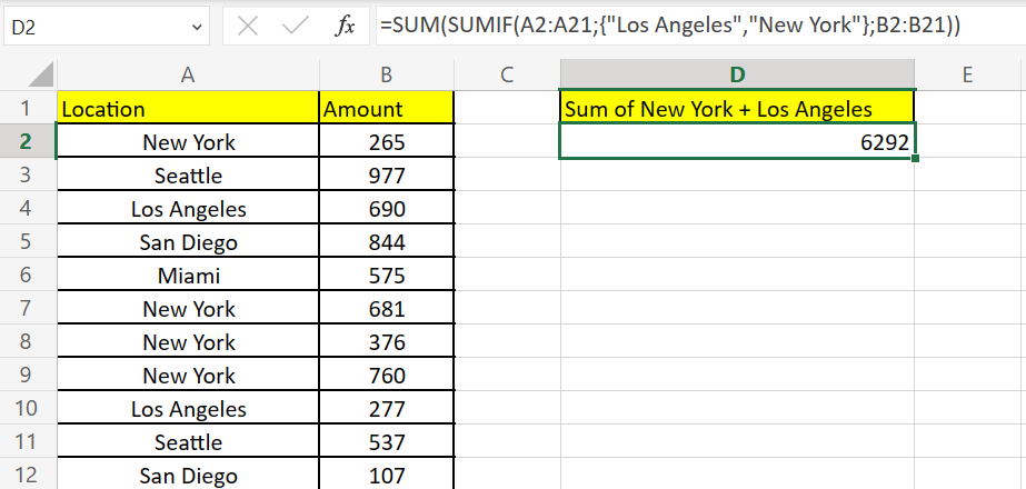
3. Hit the Enter key to evaluate the entire formula. In this example, we determined that the total transaction amount from both cities is $6292.
   
4. Another way we can add OR logic to a SUMIF formula is by using an array of criteria as an argument. The SUMIF function will return an array of results that we can add using the SUM function.
   We can start this approach by typing ‘=SUM(‘ to start the SUM function.
   
5. Next, we’ll add an instance of the SUMIF function inside our SUM function. The first argument of our SUMIF function should be the criteria range to use.
   In this example, we’ll use the Location field as our formula’s criteria range.
6. Next, we’ll add an array of acceptable values as our second argument. For example, if you want to add all values from New York and Los Angeles, we can use the array {“Los Angeles”,”New York”}.
   We’ll add the sum range as the third argument of our SUMIF function. In this example, we want to add the amounts in the cell range B2:B21.
7. You should now have a formula that uses SUMIF using an array of acceptable strings. The results of each criterion is totaled using the outer SUM function.
   
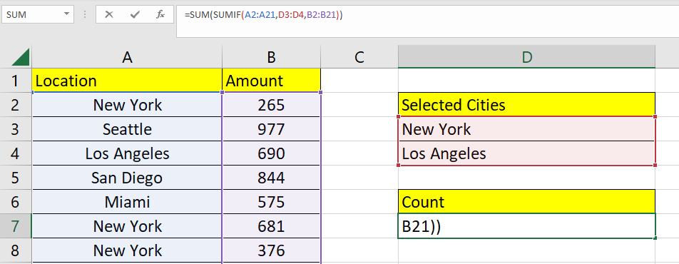
8. Lastly, we can substitute the array of criteria with an actual cell range.
   In the example above, we’ve added two cities as our target values for location.
9. Next, we’ll use the formula =SUM(SUMIF(A2:A21,D3:D4,B2:B21)) to filter out amounts with locations outside the selected cities provided in column D.
   
10. You should now have a sum of values in column B with values in column A that match the provided criteria.
    
    

This step-by-step guide should provide you with all the information you need to start using SUMIF with OR logic in Excel.

You should now have an idea of how to use the SUMIF function given a list of multiple acceptable values.

This function is just one example of the many Excel functions you can use in your spreadsheets. Our website offers hundreds of other functions and methods to help you get more out of Microsoft Excel.

With so many other Excel functions available, you can find one appropriate for your use case.

Don’t miss out on our team’s new spreadsheet tips, tricks, and best practices. Subscribe to our newsletter to stay updated on the latest guides from us!

Get emails from us about Excel.

Our goal this year is to create lots of rich, bite-sized tutorials for Excel users like you. If you liked this one, you'd love what we are working on! Readers receive ✨ early access ✨ to new content.

Subscribe