This guide will explain how to perform cluster sampling in Excel.
Excel is an excellent tool to use for performing different sampling methods. And there are many sampling methods we can use. But, we will be focusing on cluster sampling for this guide.
So cluster sampling is another common type of sampling method in which a population is divided into groups called clusters. Then, all members of some clusters will be selected to be part of the sample.
Additionally, we would usually collect groups with similar characteristics to the population being studied or focused on in cluster sampling. Ideally, we would want the clusters to be mini-representations of the population as a whole.
And cluster sampling is typically used when researchers have a hard time collecting data from the entire population as a whole. For instance, it would be difficult to collect data from every single citizen in a country.
Instead, we would consider each city as a cluster and choose a few cities to be part of the sample.
Furthermore, we could do cluster sampling easier and faster in Excel. Since Excel has several functions and tools we can use, it would be convenient to organize the population and generate a sample from it.
Let’s take another sample scenario wherein we need to perform cluster sampling in Excel.
Suppose you need to conduct a study about a new school rule which was recently passed. Since there is a large population in school and each student has a different schedule, it would be difficult to collect data from every student.
Instead, you opted to make each section a cluster and randomly choose which section would be part of your sample. And you chose to perform this process in Excel since it would make it easy to organize the data and generate the random sampling.
Before we move on, let’s first learn how to use the UNIQUE function in Excel. So this function would be used to find the unique values in the data set.
The Anatomy of the UNIQUE Function
The syntax or the way we write the UNIQUE function is as follows:
=UNIQUE(array, [by_col], [exactly_once])
Let’s take apart this formula and understand what each term means:
- = the equal sign is how we can activate any function in Excel.
- UNIQUE() refers to our
UNIQUEfunction. And this function is used to return the unique values from an inputted range or array. - array is the only required argument for this function. And it refers to the range or array which we want to return unique rows or columns from.
- by_col is an optional argument. So it refers to a logical value. If FALSE or left blank, the function will compare rows against each other and return the unique rows. If TRUE, the function will compare columns against each other and return the unique columns.
- exactly_once is another optional argument. So it is also a logical value. If TRUE, the function will return rows or columns exactly once from the array. If FALSE or omitted, the function will return all distinct rows or columns from the array.
Great! Now let’s move on and discuss a real example of how to perform cluster sampling in Excel.
A Real Example of Performing Cluster Sampling in Excel
Let’s say we have a population list containing the student IDs, the section o the student, and the number of times the student has been late or absent. And we will use this population to perform cluster sampling and generate a sample. So our initial data set would look like this:

Cluster sampling is a sampling method that splits the population into clusters and selects a few clusters to be part of the sample. In this case, we already have our clusters as sections.
So we have three clusters in the population. Afterward, we want to select two clusters to include in our sample.
Firstly, we need to find the unique values in the data set. So we will be using the UNIQUE function to identify the unique values from the Section column. In this case, we need to have three unique values since we have three clusters.
Secondly, we will type an integer starting from 1 next to each unique section name. Then, we will use the RANDBETWEEN function to select one of the integers from the list randomly.
Since the RANDBETWEEN function returns a random number between the numbers we specify, it will return a random number between 1 and 3. When the function returns a random number, we will identify which section is associated with that random number.
Afterward, the section represented by the random number will be the first cluster to be part of the sample. Next, we will return another random number using the RANDBETWEEN function.
And we will find the section associated with the second random number. So that section will be the final cluster to be included in our sample.
Next, we will filter the population list only to display the clusters that are part of the final sample. To do this, we can simply apply a filter to the data set and select the sections chosen to be part of the sample.
And our final data set would look like this:

You can make your own copy of the spreadsheet above using the link attached below.
Finally, we can explain the steps of how to perform cluster sampling in Excel.
How to Perform Cluster Sampling in Excel
In this section, we will explain the step-by-step process of how to perform cluster sampling in Excel.
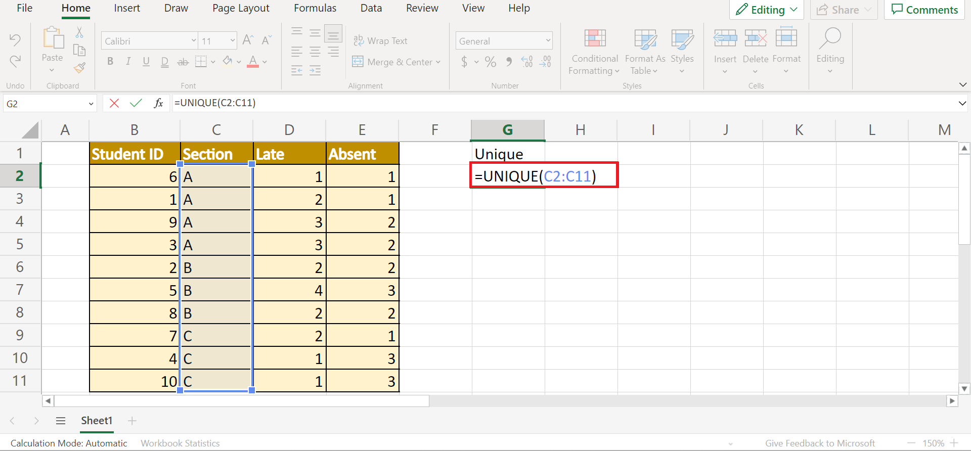
1. Firstly, we will find the unique value in a different location. In this case, we will create a Unique column. Then, we can simply input the formula “=UNIQUE(C2:C11)”. Lastly, we will press the Enter key to return the results.
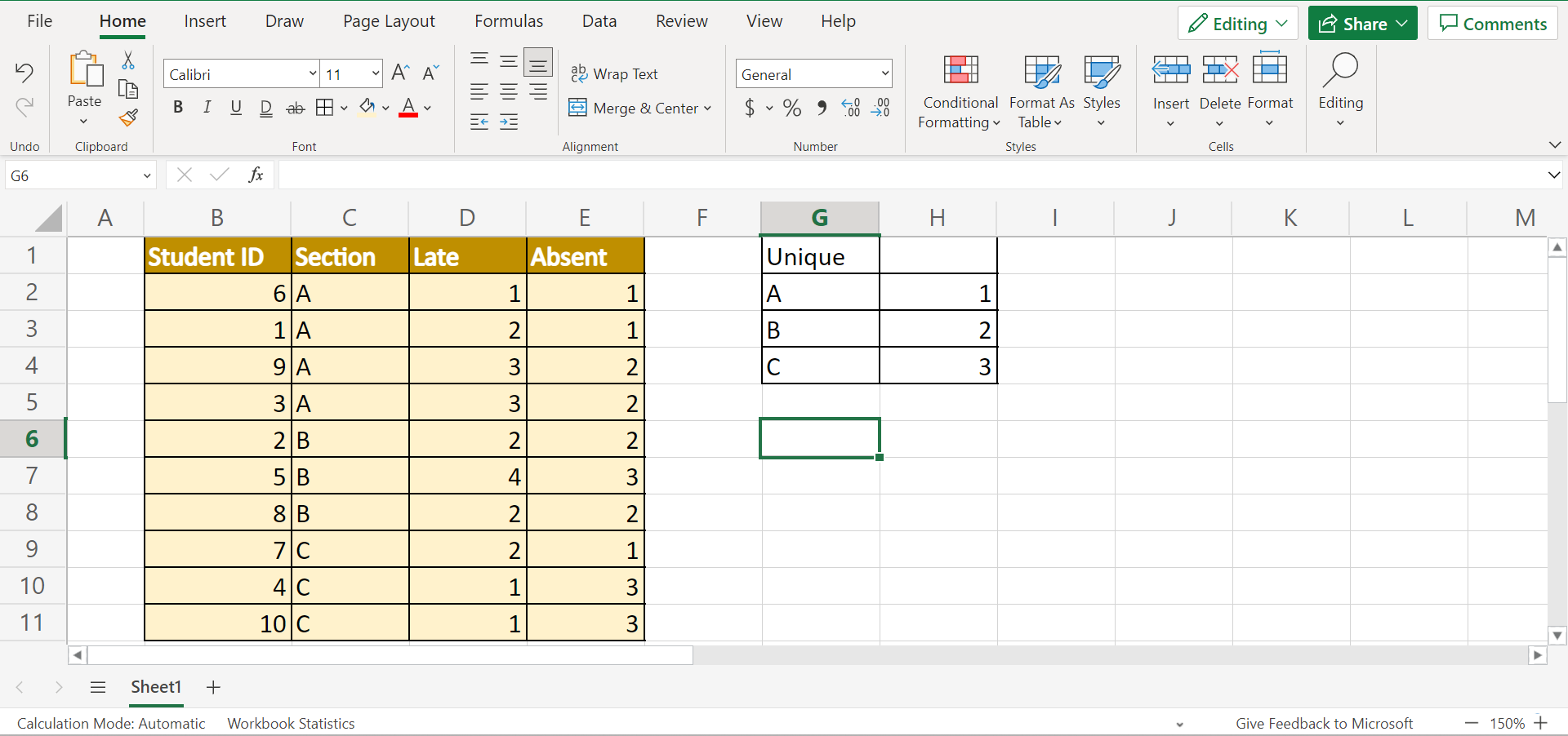
2. Secondly, we will type an integer starting from 1 for each unique value.
3. Thirdly, we need to select random clusters to include in the sample. To do this, we will use the RANDBETWEEN function. So we will type in the formula “=RANDBETWEEN(H2,H4)”. Then, we will press the Enter key to return the random value.
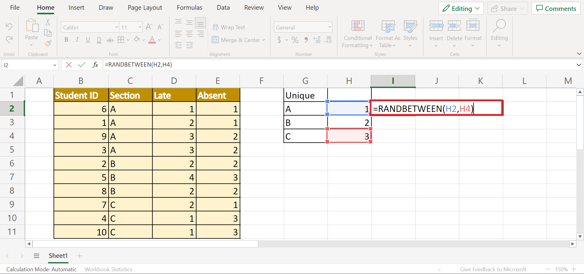
4. Next, we will identify the section associated with the random number. So this section will be the first cluster to be included in the sample. In this case, we have selected section C.

5. Afterward, we will select another random value using the RANDBETWEEN function. To do this, we simply need to select a blank cell and click Enter. And a new random value will appear.
Once again, we will find the section associated with the second random value. In this case, we have selected section B to be part of the sample.

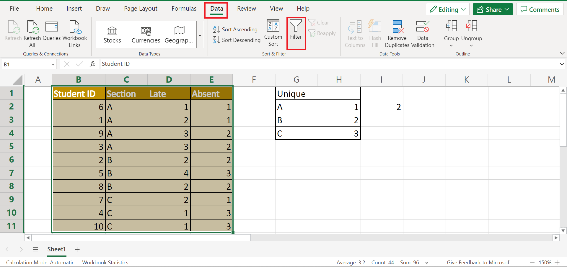
6. Then, we will filter our data set to only display our sample. To do this, we will go to the Data tab and select Filter within the Sort & Filter section.
7. Next, we will click the dropdown arrow next to the Section column. Then, we will check the boxes of sections B and C only. Lastly, click Apply.

8. And tada! We have successfully performed cluster sampling in Excel.
And that’s pretty much it! We have discussed how to perform cluster sampling in Excel. Now you can use this method in Excel whenever you need to quickly and easily generate a sample from a population using cluster sampling.
Are you interested in learning more about what Excel can do? You can now use the UNIQUE function and the various other Microsoft Excel formulas available to create great worksheets that work for you. Make sure to subscribe to our newsletter to be the first to know about the latest guides and tutorials from us.