How To Use TRUNC Function in Google Sheets

The TRUNC function in Google Sheets is useful when you need to truncate a given number to a certain number of significant digits.

Truncating a number requires omitting the less significant digits to the right of the decimal point.

The rules for using the TRUNC function in Google Sheets are as follows:

• The function requires the user to input the number to be truncated, as well as the number of digits to keep after the decimal point.
• The function then outputs the truncated number.
• TRUNC does not round the number, it only removes digits after the decimal point.

Let’s look at a quick example of a situation where we can use the TRUNC function!

Let’s say we would like to price items in a store. As a store owner, you would want to price your item with a maximum of 1 significant digit after the decimal point. For example, a bag of chips may cost $1.5 but not $1.49. There are also cases where applying discounts leads to a long decimal, which you would like to avoid. How do you make sure that the prices fit your requirements?

Using the TRUNC function, it becomes quite easy to truncate prices to a certain number of significant digits.

This use case is just one example of when we can use the TRUNC function in Google Sheets. Significant figures are an important thing to consider when working with calculations in the sciences, and may also be useful in financial use-cases.

Now that we understand when to use the TRUNC function, let’s go into how we can write it on Google Sheets.

The Anatomy of the TRUNC Function

The syntax of the TRUNC function is as follows:

=TRUNC(value, [places])

Let’s dissect this thing and understand what each of these terms means:

• = the equal sign is how we start any function in Google Sheets.
• TRUNC() is our TRUNC function. The function truncates a given number according to a specified number of places and returns that truncated number.
• value refers to the actual number that we want to truncate.
• places refers to the number of significant digits to the right of the decimal point to retain.
• If the value of places is greater than the number of significant digits in value, then no modification is done.
• If the value of places is negative, the specified number of digits to the left of the decimal place is changed to zero. For example, =TRUNC(124.5,-2) will return 100, with the “24” converted to zeroes.
   

A Real Example of Using TRUNC Function

Let’s look at a few examples of the TRUNC function being used in a Google Sheets spreadsheet.

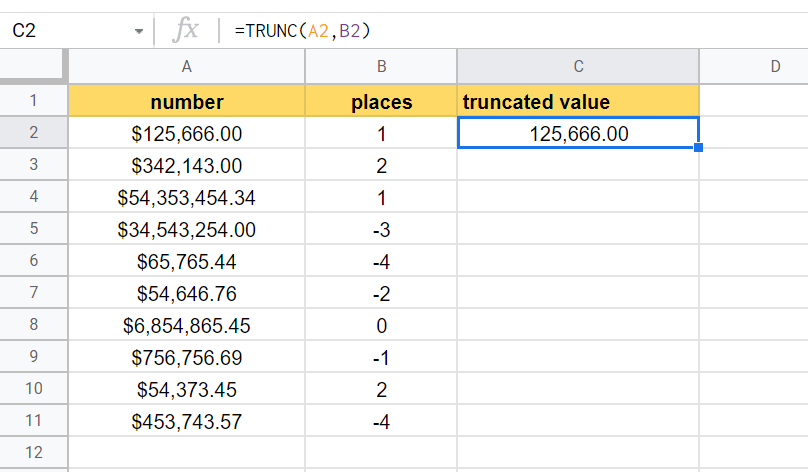
In the table below, we have a data set of prices with a varying number of significant digits. In columns B through C, we use the TRUNC function to truncate to a specified number of digits.

To get the values in Column C, we just need to use the following formula:

=TRUNC(A2,1)

You can make a copy of the spreadsheet shown above using the link I have attached below. 

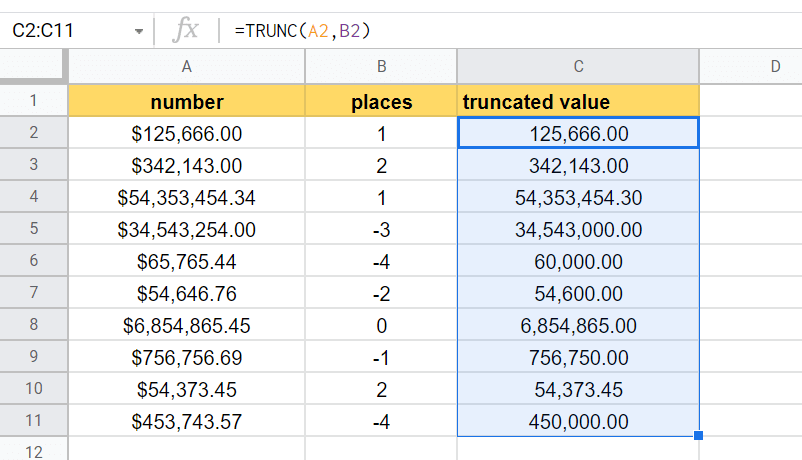
In the second example below, we can see how we can use TRUNC to remove significant digits to the left of the decimal as well. Using negative numbers in our places argument allows us to truncate digits in the ones, tens, and hundreds of places and beyond.

If you’re ready to try out the TRUNC function in Google Sheets, let’s move on to the next section to learn how we can apply it on an actual spreadsheet.

How to Use TRUNC Function in Google Sheets

1. First, we should select the cell to type in our TRUNC function. In this example, we’ll start with cell C2.
   
   
   
   
2. Next, we need to type in the equal sign ‘=‘ to begin the function, followed by ‘TRUNC(‘. 
3. A tooltip box appears with information about the TRUNC function. We can click on the arrow found in the top-right-hand corner of the box to minimize it.
   
   
   
   
4. For the next step, we need to fill in our arguments. Our value to be truncated is found in Column A, and the number of places to truncate is specified in Column B.
   After filling in our arguments, simply hit the Enter key on your keyboard to let the function return the result.
   
   
   
   
5. Finally, we can drag down the formula in cell C2 to fill the rest of the table!
   
   
    

Frequently Asked Questions (FAQ)

1. What is the difference between TRUNC and ROUND function?
   While both functions modify the decimal places of numbers in Google Sheets, their functions are slightly different. TRUNC simply removes significant digits while ROUND follows the standard rules of rounding. The TRUNC function will never round up a decimal.
    
2. What is the difference between TRUNC and INT functions?
   Without any place argument, TRUNC works roughly the same as the INT function. Comparing both functions, the TRUNC function is much more powerful since you can specify the number of places to retain after the decimal point.

This step-by-step tutorial shows how easy it is to use the TRUNC function to remove significant digits in a number. You can now use the TRUNC function in Google Sheets together with the many other Google Sheets formulas available to create more powerful worksheets.

If you found this guide helpful, do consider subscribing to our newsletter to stay notified of new guides like this.

Get emails from us about Google Sheets.

Our goal this year is to create lots of rich, bite-sized tutorials for Google Sheets users like you. If you liked this one, you'd love what we are working on! Readers receive ✨ early access ✨ to new content.

Subscribe