A Value at Risk template in Excel is useful when you need to find out the potential loss in your portfolio over a given period at a given confidence interval.
One of the simplest ways to calculate Value at Risk is through the use of the normal distribution.
While VaR assumes that the investment returns have a normal distribution, actual investments are usually fat-tailed and skewed away from a normal distribution.
Similarly, VaR can only work as well as the confidence level used to compute it. A VaR of $1M at a confidence level of 95% tells you that you might experience this loss in 5 out of every 100 trading days.
Let’s take a look at a quick scenario where we can use a Value at Risk template to quantify financial risk.
Suppose you have an investment portfolio worth $10,000. The average return for a single day is 0.12. With a 99% confidence level, what is the value at risk for a single time?
First, we must look for the minimum expected return with respect to the given confidence level. We can use the NORM.INV function to get this value. Once we obtain this value, we can then calculate the Value of the Portfolio given the minimum expected returns.
The difference between this amount and the original value of our portfolio is the Value at risk.
Now that we know the purpose of using a Value at Risk template, let’s take a look at how it works on a spreadsheet.
A Real Example of a Value at Risk Template in Excel
Let’s take a look at a real example of a spreadsheet with a Value at Risk template.
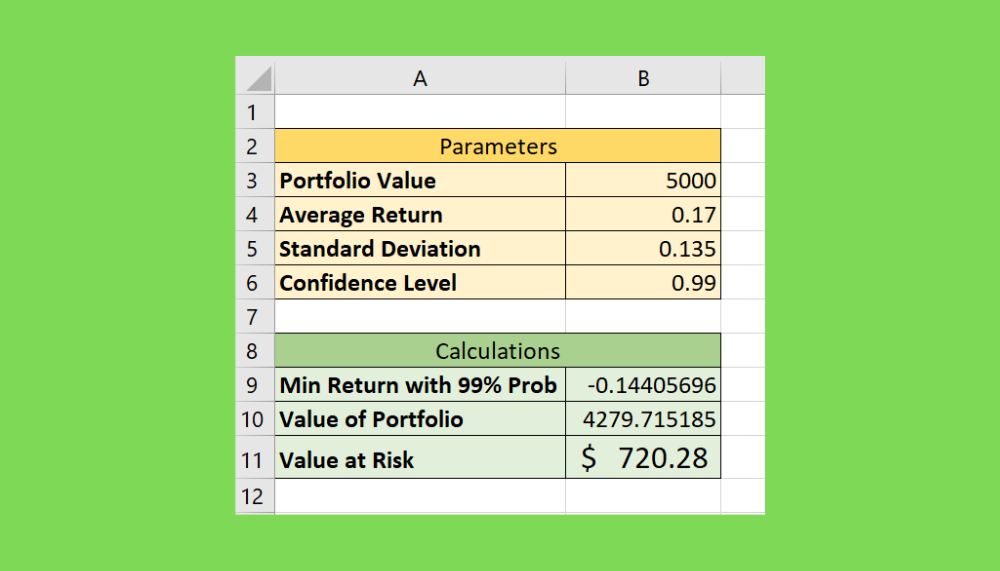
In the table below, our template is divided into two sections. The parameters table contains our input. The user must provide the portfolio value, average return, standard deviation, and desired confidence level.

These inputs are then used to calculate the Value at Risk. First, we use the NORM.INV function to calculate the minimum returns given the 99% probability.
To get the value in cell B9, we use the following formula:
=NORM.INV(1-B6,B4,B5)
Once we get the minimum returns, we can then compute the value of the portfolio with those returns. We can obtain the value in cell B10 through this formula:
=B3*(B9+1)
Lastly, to compute the Value at Risk, we must find the difference between this new value of the portfolio with the original input portfolio value.
=B3-B10
You can make your own copy of the spreadsheet above using the link attached below.
If you’re ready to create your own Value at Risk template in Excel, read our step-by-step guide in the next section!
How to Create a Value at Risk Template in Excel
This section will explain each step needed to create a Value at Risk template in Microsoft Excel. You’ll learn how we can use this template to compute the potential loss of an investment in a given time.
Follow these simple steps to add a Value at Risk template to your spreadsheet:
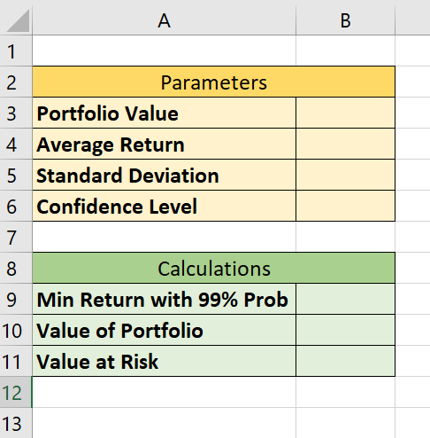
- First, you should have the following tables set up. The first table is where the user places the input of the VaR template. The second table will have the formulas used to compute the Value at Risk.
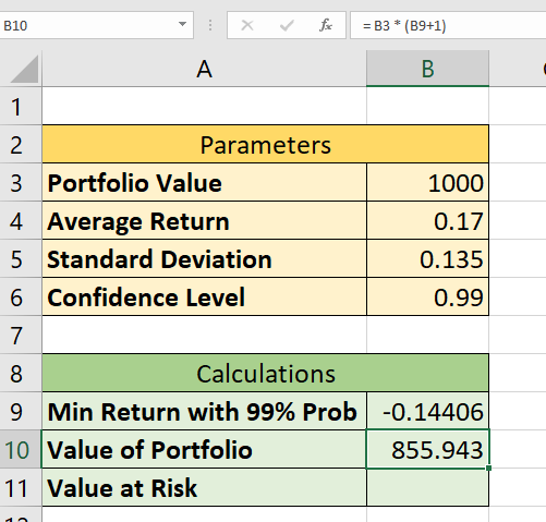
- Next, input the indicated values in the Parameters table. For this example, we have a portfolio value of $1000 with an average return of 0.17 and a standard deviation of 0.135. We’ve also indicated that we want the VaR to have a confidence level of 99%.

- Now that we have the input, we can start calculating some important metrics. First, we’ll need to find the minimum return of our investment with the given confidence level. We can use a
NORM.INVformula to get our returns.

- Next, we can use the value returned in the previous step to compute the new value of the portfolio.
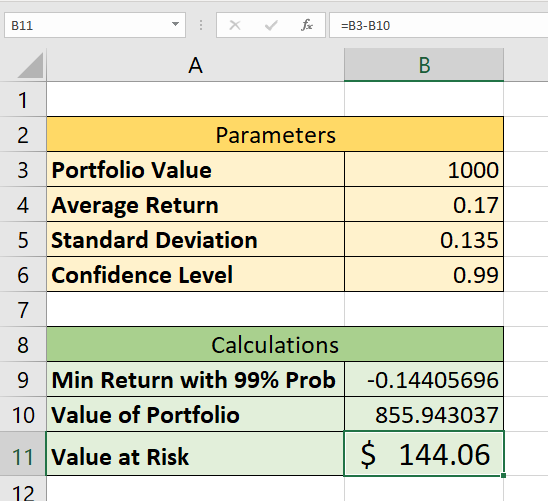
- To get the Value at Risk, we must find the difference between the new value of the portfolio and the original value. In this example, we’ve received a minimum return of $855.94 from our original value of $1000. This gives us $144.06 as our VaR.
Frequently Asked Questions (FAQ)
- How do I calculate my VaR over a given month?
The step-by-step guide covers a case where the time is a single day. To get the VaR over a month, simply multiply the Value at risk for a day by the square root of the number of trading days in a month.
For example, let’s say my daily VaR is $100, and there are 22 trading days in a month. Computing for my monthly VaR should be=SQRT(22) * 100which is equal to $469.04
That’s all you need to remember to create your own Value at Risk template in Excel. This step-by-step guide should be all you need to compute the extent of possible financial losses in a portfolio over a specific time frame.
Value at Risk is just one example of a financial measure that you can compute in Excel. With so many other Excel functions out there, you can surely find one that best suits your use case.
Are you interested in learning more about what Excel can do? Make sure to subscribe to our newsletter to be the first to know about the latest guides and tutorials from us.