


This guide will explain how to create a frequency distribution in Microsoft Excel.
We can use the FREQUENCY function and the PivotTable feature in Excel to analyze the spread of our data across different intervals.
A frequency distribution table is a helpful statistical method showing users the mean and variance of a particular dataset.
Suppose we were to conduct a random survey of people visiting a particular store. We want to know which age range frequents this store the most.
Given an Excel dataset of age values, we can use the FREQUENCY function to create a frequency distribution table that counts how many respondents fall under different age groups. We can also use the PivotTable tool to generate a similar view of our data.
Now that we know what tools to use to create a frequency distribution table, let’s take a look at a working example on an actual spreadsheet.
A Real Example of Creating a Frequency Distribution in Excel
The following section will provide a few methods users can follow to create a frequency distribution in Excel. We will also explain the formulas and tools used in these examples.
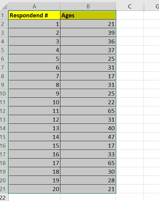
First, let’s take a look at our sample data. Our dataset of 20 respondents from a survey includes data about their age. We want to create a frequency distribution table to determine how the population is spread across different age groups.
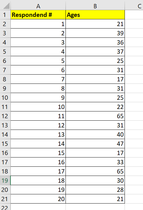
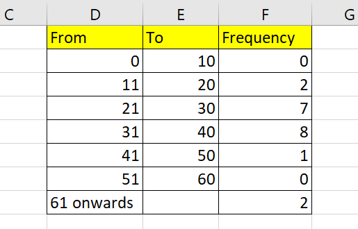
We can create a frequency distribution table that defines the different age groups or classes to consider in ascending order. For example, the first age group will contain all respondents aged 0 to 10. The last age group will include all respondents aged 61 and onwards.
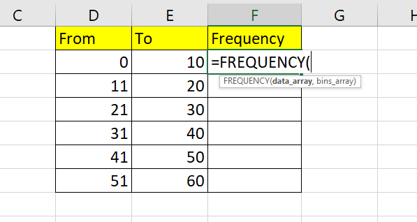
To get the values in Column C, we just need to use the FREQUENCY formula in cell F2:
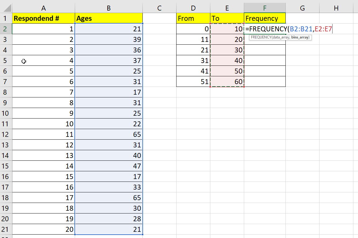
=FREQUENCY(B2:B21, E2:E7)
The FREQUENCY function accepts two arguments to generate the frequency distribution. The first argument will be the range or set of values for which you want to count the frequencies. The second argument will indicate the intervals to use for grouping the individual values.
In our example, we’ve set our first argument to B2:B21 since it contains all the ages of our respondents. Next, we’ve set the range E2:E7 as our second argument to set up the different age groups we want to group our respondents in.
Based on the FREQUENCY function, we can now determine that the age range of 31-40 contains the most number of respondents.
We can also create a frequency distribution table using Excel’s PivotTable feature.

An advantage of using PivotTables for creating frequency distribution is that users are able to keep track of more metrics at once. Users also no longer need to manually enter the values needed to define the intervals of each grouping.
Do you want to take a closer look at our examples? You can make your own copy of the spreadsheet above using the link attached below.
Use our sample spreadsheet to test out how we created a frequency distribution table using both methods seen earlier.
If you’re ready to create your own frequency distribution table in Excel, head over to the next section to read our step-by-step breakdown on how to do it!
How to Create a Frequency Distribution in Excel
This section will guide you through each step needed to create a frequency distribution table. You’ll learn how to use the built-in FREQUENCY function with user-defined intervals. You will also see how to create a frequency distribution table through Excel’s PivotTable feature.
Follow these steps to start adding a frequency distribution in Excel:
- First, we’ll create a frequency distribution with the
FREQUENCYfunction.
The user must create a new table that outlines the different intervals to calculate the frequency distribution.
 In the example above, the values in column E are the most important. These values determine the upper limits of each grouping used for the frequency distribution output.
 - Next, type the formula “=FREQUENCY(“ to start the
FREQUENCYfunction.
- Enter the range you want to find the frequencies for as the first argument.

- Next, enter the array that we’ll use to define the intervals.
 In this example, we’ll use the range E2:E7.
 - Hit the Enter key to evaluate the
FREQUENCYfunction. The function should return an array of values corresponding to the number of values found in each grouping.
Do note that an additional element will appear in the output. This value is a count of all values above the highest interval. In this example, two respondents are over 60, our highest specified interval. - We can also calculate frequency distribution using the PivotTable feature.
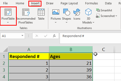
First, select the dataset in your spreadsheet.
- In the Insert tab, click on the PivotTable option.
- Drag the field you want to calculate the frequency of into both the Rows and Values areas.
 Ensure that the Values field uses the Count aggregation.
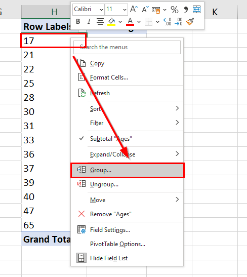
 - Right-click on the row label and select Group…
- In the Grouping dialog box, users can set parameters such as the size of the group.
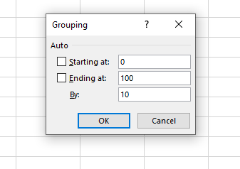 Click on OK to proceed.
 - The row labels of your frequency distribution should now show the generated groupings, and the sole values column will display the frequency or count for each group.
These are all the steps needed to create a frequency distribution in Excel.
This step-by-step guide should be a quick and straightforward introduction to creating your own frequency distribution table in Microsoft Excel.
We’ve shown you how to find the frequencies of a range of values using the FREQUENCY function and user-defined intervals. Our guide also explained how to use the PivotTable feature to create a frequency distribution of your dataset in a few clicks.
The FREQUENCY function just one example of the many Excel functions you can use in your spreadsheets. Our website offers hundreds of other functions and methods to help you get more out of Microsoft Excel.
With so many other Excel functions available, you can find one appropriate for your use case.
Don’t miss out on our team’s new spreadsheet tips, tricks, and best practices. Subscribe to our newsletter to stay updated on the latest guides from us!


