


This guide will discuss how to perform a left join in Excel using two simple and efficient methods.
Since Excel contains many tools and functions that make performing tasks easier and faster, it is a popular tool for organizing data. And it has many tools we can use to manipulate and organize different data sets.
And one thing we can perform in Excel is a left join. So a left join is used to join together two tables so that every row in the left table is kept and returned. Then, only the rows with a matching value in a specific column of the right table are kept and returned.
Unfortunately, Excel does not have a built-in function we can utilize that is solely for left join. However, we can use other tools to perform a left join.
Firstly, we can use the VLOOKUP function to perform a left join in Excel. Secondly, the merge dialog box in the power query editor has several join kinds available. And, of course, one of these is a left outer join which we can use.
Let’s take a sample scenario wherein we must perform a left join in Excel.
Suppose you are organizing your data. So you have two data sets that are slightly similar. And you want to create just one data set for both tables. In this case, the left data set contains all information you need. But, there is one column in the right table you also need.
To solve this issue, you opted to perform a left join to merge the two tables and keep only the specific column from the right table.
Great! Now let’s move on and dive into a real example of performing a left join in Excel using two easy and efficient methods.
A Real Example of Performing a Left Join in Excel
For instance, we have two data sets with similar information. On the left side, we have a data set containing the employee name and the employee ID. Then, we have our second data set, which has the same employee ID and the department they work in.
So our initial data set would look like this:
Since we need to create a single data set containing all the columns from the left table and just one column from the right table, it would be best to perform a left join. And we can utilize two methods to accomplish this.
Firstly, we can utilize the VLOOKUP function to do a left join in Excel. So a VLOOKUP function is used to look for a value in the leftmost column of a selected table. Then, the function will return a value in the same row from another column we specify.
Essentially, VLOOKUP will search for a match in the lookup value we select and return the match from the selected column. And we can use this function to return the column we need from the right table and join them together with our left table.
Firstly, we can copy and paste the left table into a new location. Next, we will use the VLOOKUP function to search for a match using the employee ID. Then, we will return the department column to join the left table we have copied and pasted.
Secondly, we can also use the left outer join option in the Merge dialog box in the power query editor. So power query in Excel is usually used to import or connect tables to external data. Then, we can manipulate that data to our preference. For example, we can merge tables or remove a column.
In this case, we want to use the left outer join option. Firstly, we need to convert the data sets into tables. Then, we will go to the merge queries. Afterward, we will select the necessary columns in the merge dialog box and select the left outer option under the join kind section.
Finally, this is what our final data set would look like after using any of the two methods to perform a left join in Excel:

You can make your own copy of the spreadsheet above using the link attached below.
Amazing! Now let’s learn the steps of how to perform a left join in Excel using two simple and efficient methods.
How to Perform a Left Join in Excel
In this section, we will explain the step-by-step process of how to perform a left join in Excel. Furthermore, each step will have detailed instructions and pictures for you to follow easily.
1. Firstly, we will use the VLOOKUP function to perform a left join. But, we first need to create a copy of the left data set. So we need to select the left data set and press Ctrl + C to copy. Then, we will select a new location and press Ctrl + V to paste the table.
Otherwise, we can also right-click and choose Paste in the menu.

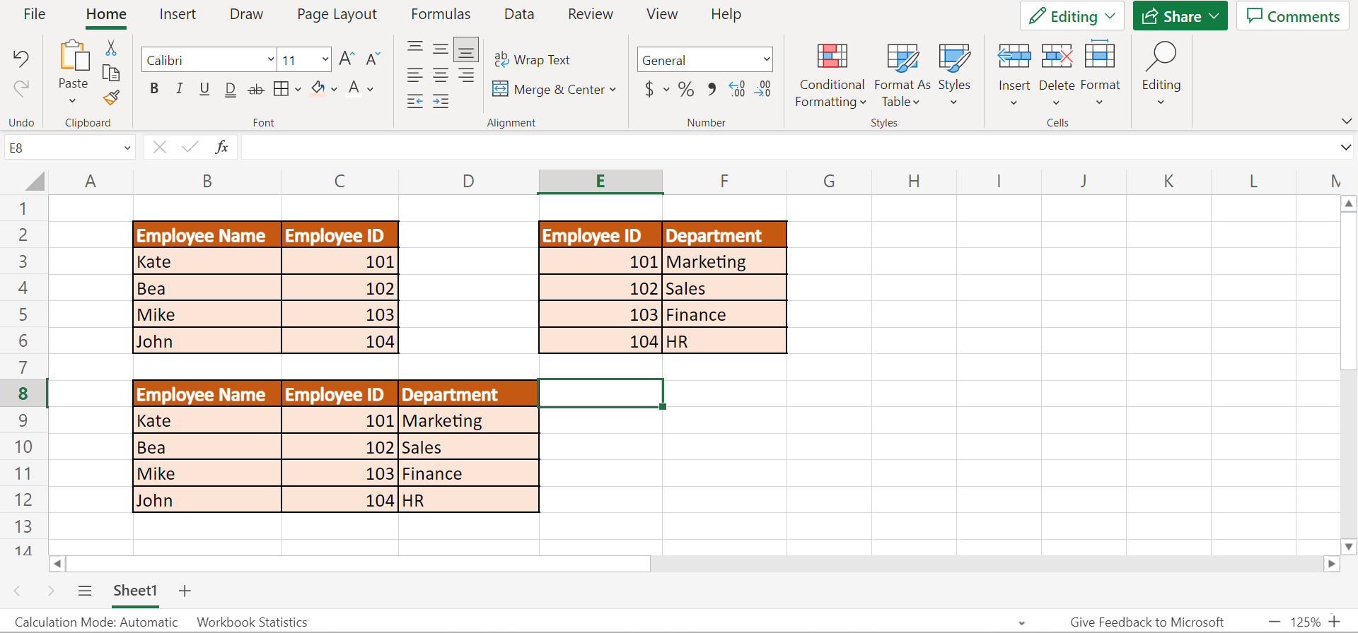
2. Secondly, we will now use the VLOOKUP function to perform a left join. So we will start the formula with an equal sign beside the copied left data set. In this case, we will type in the formula “=VLOOKUP(C3,$E$3:$F$6,2, FALSE)” in cell D9. Then, press the Enter key to return the results.
Moreover, we can add a header for the returned column to fix our data set.

3. And tada! We have successfully used the VLOOKUP function to perform a left join in Excel.
4. Next, let’s try using the power query to do a left join. Firstly, let’s convert our two data sets into tables. To do this, select the data set and go to the Insert tab. Then, select Table.

5. Then, we have to name each table. So we will select any cell in the table and go to the Table Design tab and change the name to something unique and meaningful.

6. Afterward, we will go to the Data tab and select From table/Range to form a connection.

7. Next, we will go to the Home tab in the Power Query Editor and select Close & Load. Then, we will click Close & Load To in the dropdown menu.

8. Once the Import Data dialog box is open, we will choose Only Create Connection. And we will repeat the same process to the right table.

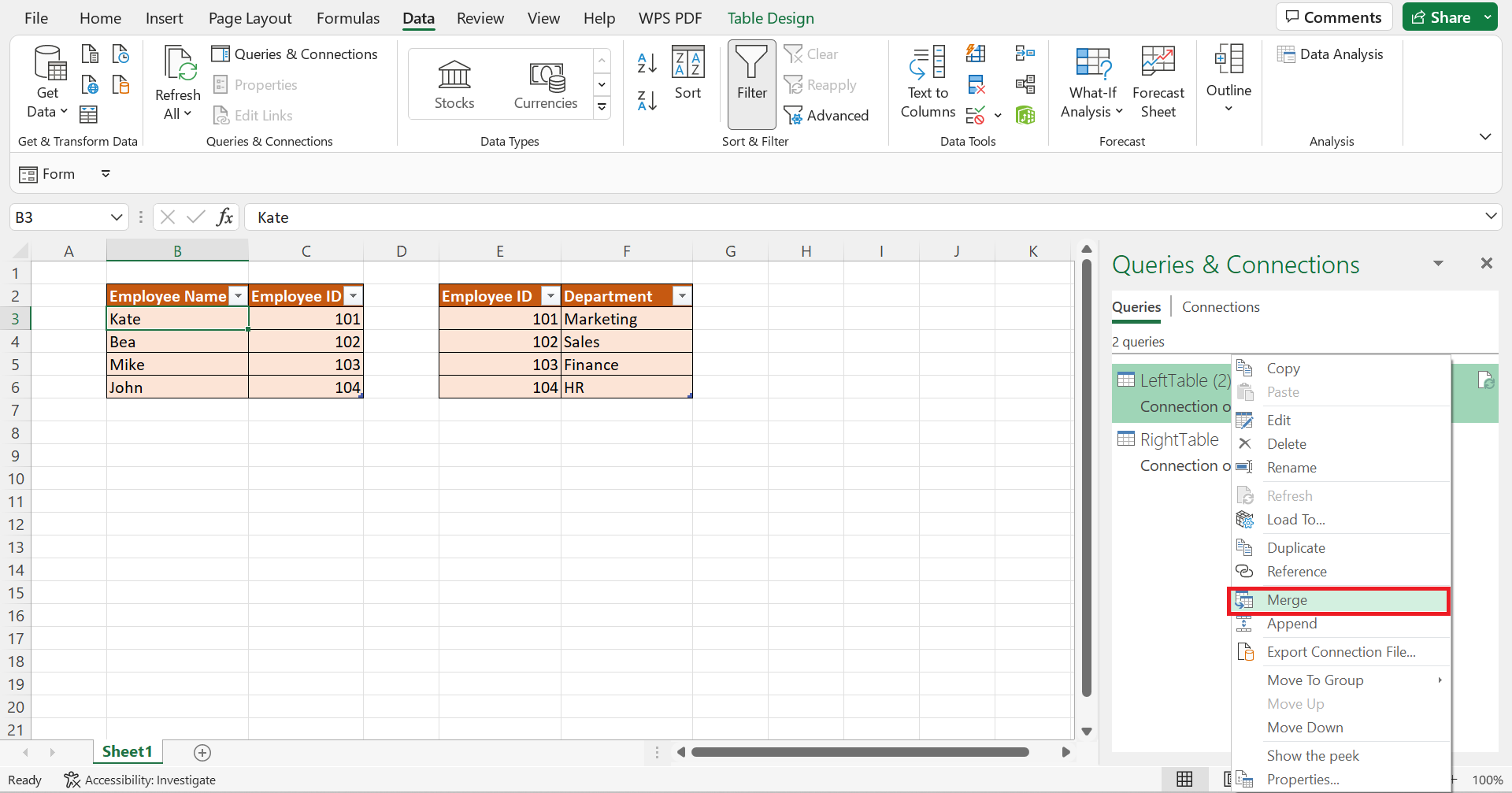
9. After creating the connections, go to the Queries & Connections opened at the side. Then, we will right-click the LeftTable and click on Merge.
10. When the Merge dialog box opens, we need to select the LeftTable on the first preview and select the Employee ID column. Then, we will select the right table on the second preview and select the Employee ID column.
Then, we will select the Left Outer in the Join Kind section. Finally, click OK to apply the merge.

11. Next, we will click the expand field to display the values on the column. And we will select only the Department. Finally, click OK.

12. Afterward, we will click Close & Load. Then, select Close & Load To.

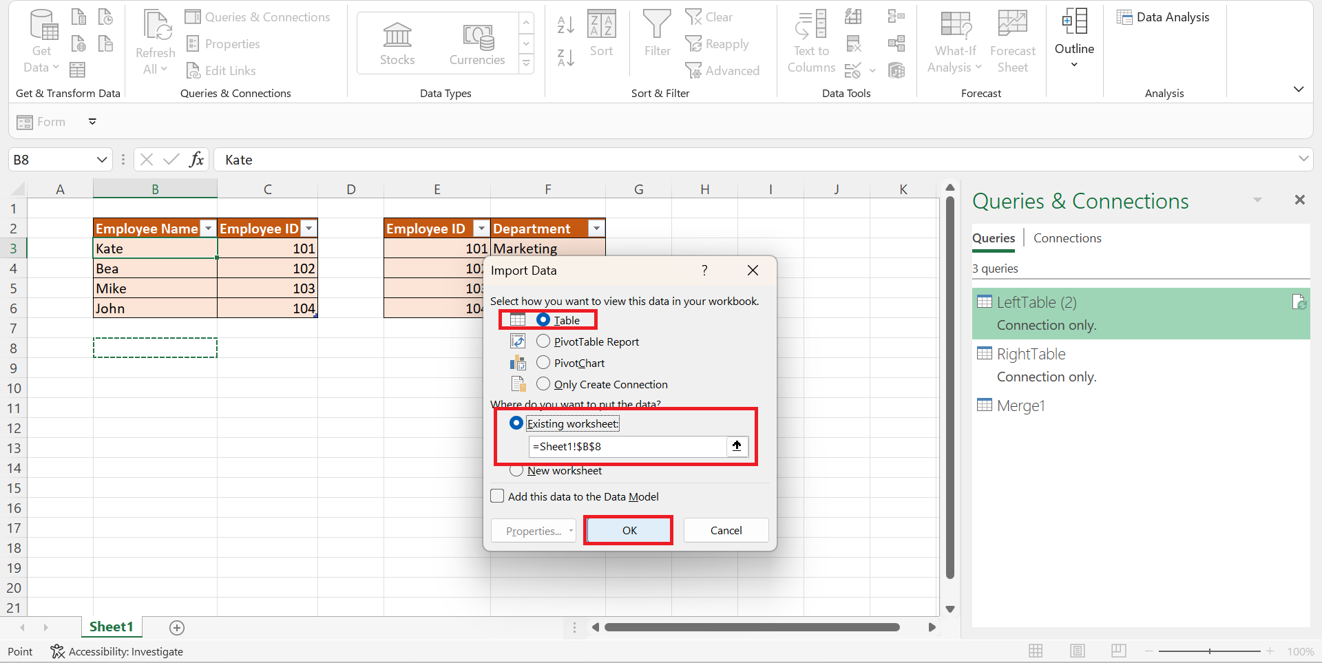
13. To display our new table, we will select Table and Existing Worksheet. Lastly, we will click select OK to apply.
14. And tada! We have finally performed left join in Excel using the left outer join in the power query.
And that’s pretty much it! We have explained how to perform a left join in Excel using two simple and efficient methods. Now you can choose any of the two methods and apply them to your work whenever you need them.
Are you interested in learning more about what Excel can do? You can now use the VLOOKUP function and the various other Microsoft Excel formulas available to create great worksheets that work for you. Make sure to subscribe to our newsletter to be the first to know about the latest guides and tutorials from us.


