How to Use LOGEST Function in Excel

This guide will explain how to use LOGEST function in Excel.

The rules for using the LOGEST function in Excel are the following:

• The LOGEST function calculates the exponential curve that fits your data. Then, the function will return an array of values that describes the curve. 
• We must enter the function as an array formula. Otherwise, the function will only return the first m value in the calculated array. 
• When the array known_ys is in a single column, the function will interpret each column of known-xs as separate variables.
• When the array known_ys is in a single row, the function will interpret each row as separate variables.
• When we only input one variable in known_xs, the known_ys and the known_xs can be ranges of any dimensions as long as they have equal dimensions.
• If const is TRUE or left blank, the b is calculated normally.
• If const is FALSE, the b is set equal to 1 while the m-values will be fitted to y = m^x.

Excel is an excellent tool to use when performing different calculations. Since it has several built-in functions and tools we can utilize, we can easily and accurately do complex and long calculations.

However, we will focus on the LOGEST function, which we can utilize to find the exponential curve that fits our data. So the LOGEST function is most often used during regression analysis. 

Let’s take a sample scenario wherein we need to use the LOGEST function in Excel.

Suppose you have a data set containing different values for x and y. And you want to calculate the exponential curve that will fit your data set best. Then, you want to return an array of values describing the curve. 

To do this, you utilized the LOGEST function in Excel. With the help of the LOGEST function, you easily determine the statistical information on the exponential curve of best fit through the given x and y values in the data set.

Before we move on to a real example of using the LOGEST function in Excel, let’s first learn how to write and use the function.

The Anatomy of the LOGEST Function

The syntax or the way we write the LOGEST function is as follows:

=LOGEST(known_ys,[known_xs],[const],[stats])

Let’s take apart this formula and understand what each term means:

• = the equal sign is how we start any function in Excel.
• LOGEST() refers to our LOGEST function. And this function is used to return the statistics that describe an exponential curve matching the known data points in the data set.
• known_ys is a required argument. So it refers to the set of y-values that is already known in the relationship y = b*m^x.
• known_xs is an optional argument. And it refers to the optional set of x-values that is already known in the relationship y = b*m^x.
• const is another optional argument. So it refers to a logical value that will dictate how b is calculated. If TRUE or left blank, b will be calculated normally. Otherwise, b will be set equal to 1.
• stats is also an optional argument. And this refers to a logical value that will dictate what other information is returned. When the stats is TRUE, the function will return additional regression statistics. When it is FALSE or omitted, the function will return m-coefficients and the constant b. 

Great! Now we can move on and dive into a real example of using the LOGEST function in Excel.

A Real Example of Using LOGEST Function in Excel

Let’s say we have a data set containing x and y values. So our initial data set would look like this:

So the LOGEST function in Excel is based on the equation of the curve, which is y = b*m^x. Before we go and use the LOGEST function in Excel, we will first verify that the values in our data set actually follow an exponential curve. To do this, we will quickly insert a scatter plot of x versus y.

Once we can see that the data follows an exponential curve, we can use the LOGEST function in Excel. Firstly, we will utilize the function to find the exponential curve formula. 

So the first value returned will represent the value for m while the second value in the returned output will represent the value for b in the equation y = b*m^x.

Then, we can input the returned values in the formula to predict the values of y based on the x-values.

For example, we assume that the value of x is 5. Since we already used the LOGEST function, we have the value of b, which is 2.561581315, and the value of m, which is 1.439448993. Afterward, we can use this formula to predict that y has a value of 15.83031466 when x has a value of 5. 

Additionally, we can also display additional statistical information aside from the values of b and m. To do this, we simply set the logical value TRUE for the stats argument in the LOGEST function.

Thus, we will receive more statistical information. So the LOGEST function will return information about the standard error for m and b, the R^2 of the model, the standard error for y, the F-statistics, the degrees of freedom, the regression sum of squares, and the residual sum of squares. 

So our final data set would look like this:

You can make your own copy of the spreadsheet above using the link attached below. 

Amazing! Now we can proceed and explain the steps of how to use the LOGEST function in Excel.

How to Use LOGEST Function in Excel

In this section, we will explain the step-by-step process of how to use the LOGEST function in Excel. Additionally, each step contains detailed instructions and pictures to help you along the way.

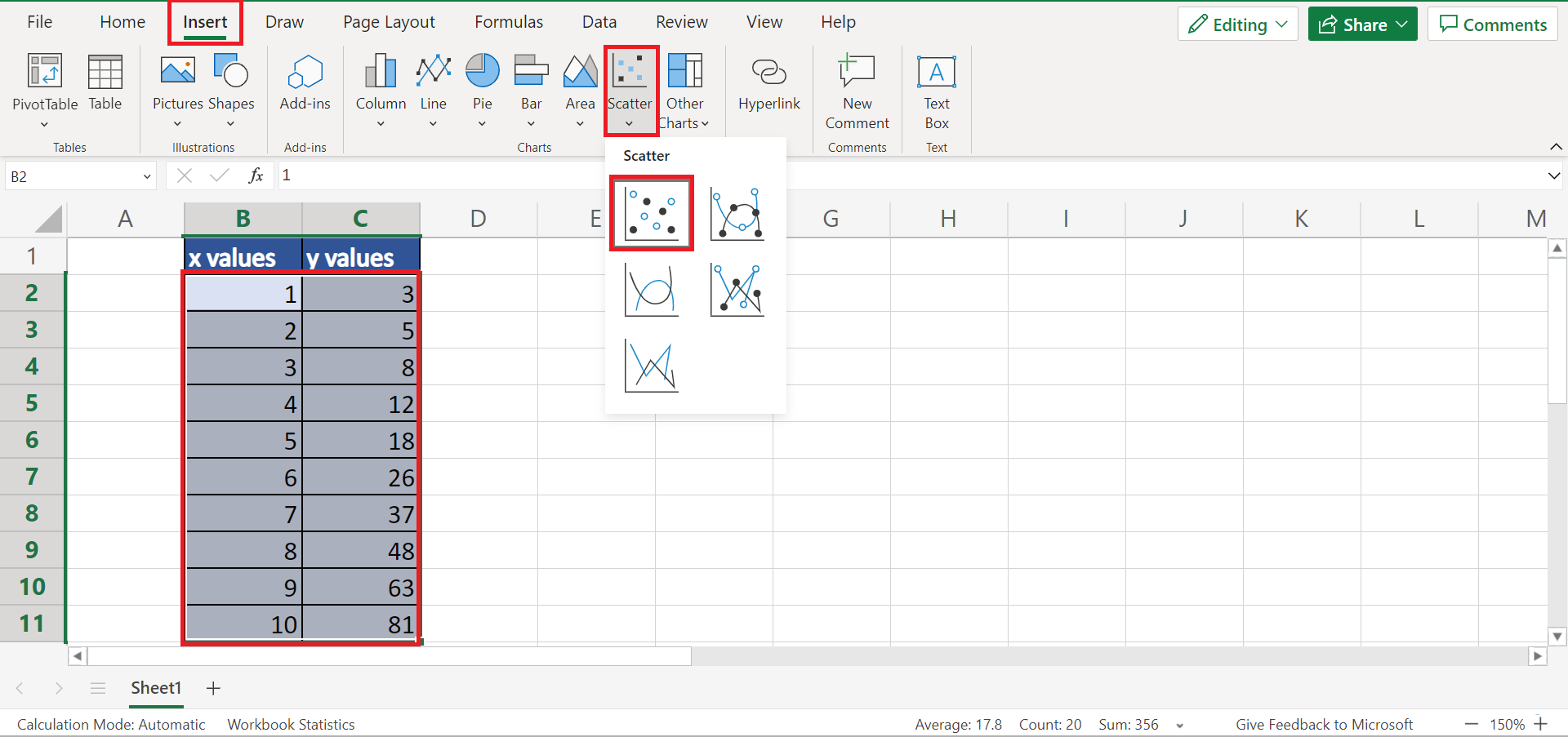
1. Firstly, we need to verify that the x and y values in our data set follow an exponential curve. To do this, we will select the data set and go to the Insert tab. Then, we will select Scatter and click the Scatter with Only Markers icon in the dropdown menu.

2. Once the chart has been inserted, we can now verify that our data set does actually follow an exponential curve.

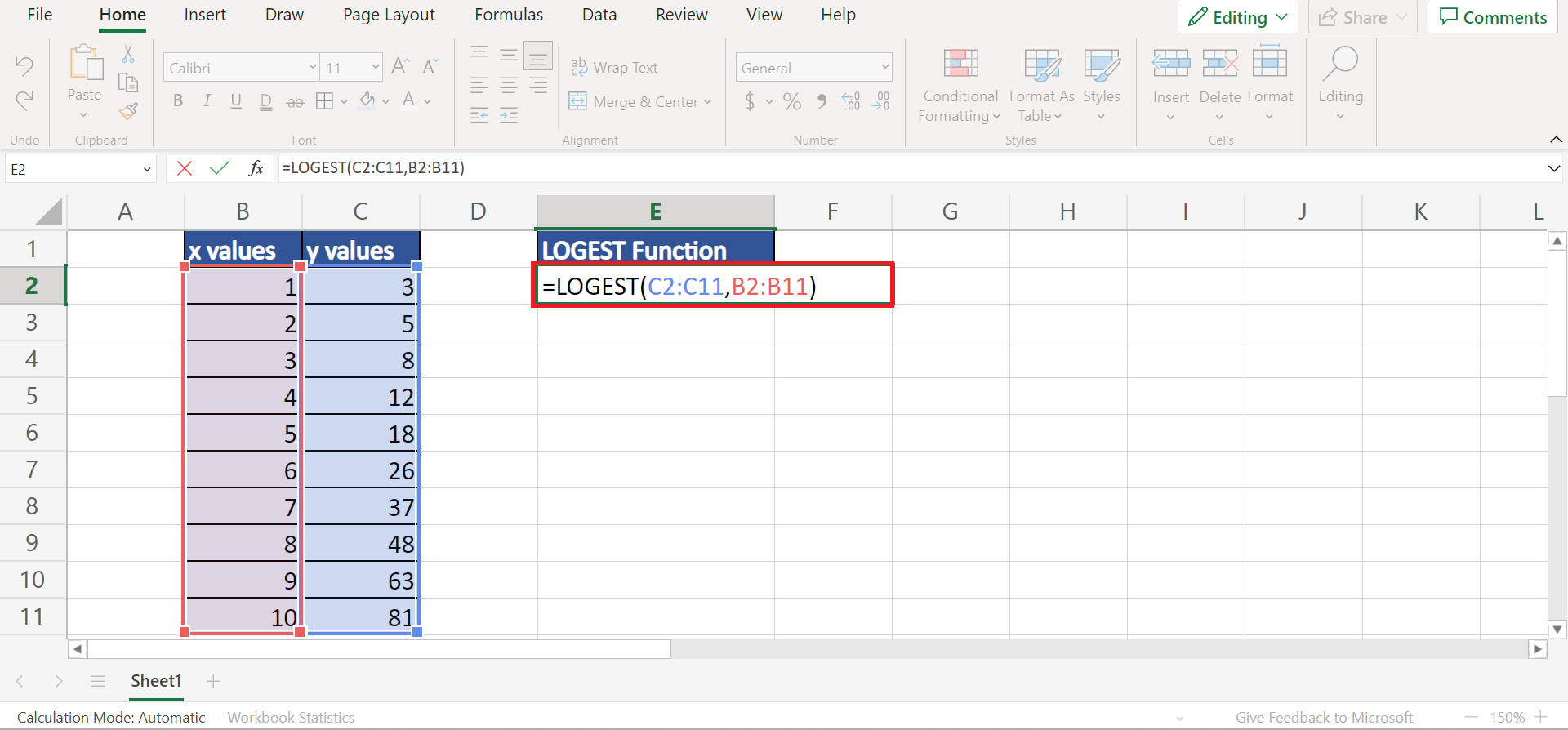
3. Next, we can now use the LOGEST function to get the exponential curve formula. In this case, we will type in the formula “=LOGEST(C2:C11,B2:B11)”. Lastly, we will press the Enter key to return the result.

4. Using the returned output, we can predict the value of y. For instance, let’s assume x has a value of 5. So we will input the returned values in the formula “=F2*E2^5”. Lastly, we will press the Enter key to get the result.

5. Additionally, we can display additional regression statistics by setting the stats argument in the function as TRUE. To do this, we will type in the formula “=LOGEST(C2:C11,B2:B11,,TRUE)”. Lastly, we will press the Enter key to return the information.

6. And tada! We have successfully used the LOGEST function in Excel.

And that’s pretty much it! We have explained how to use the LOGEST function in Excel. Now you can go ahead and apply this to your work.

Are you interested in learning more about what Excel can do? You can now use the LOGEST function and the various other Microsoft Excel formulas available to create great worksheets that work for you. Make sure to subscribe to our newsletter to be the first to know about the latest guides and tutorials from us.

Get emails from us about Google Sheets.

Our goal this year is to create lots of rich, bite-sized tutorials for Google Sheets users like you. If you liked this one, you'll love what we are working on! Readers receive ✨ early access ✨ to new content.

Subscribe