The CRITBINOM function in Google Sheets is useful when you need to calculate the smallest value for which the cumulative binomial distribution is greater than or equal to a given criteria.
This function can be used to return the smallest number of successes to reach a success threshold given a certain criteria. This is also known as the critical value of a cumulative binomial distribution.
The rules for using the CRITBINOM function in Google Sheets are as follows:
- The function requires three arguments: the number of independent trials, the probability of success for each trial, and the desired threshold probability.
- The function then outputs the critical value of the distribution.
Let’s begin with understanding what a binomial distribution refers to.
Binomial distribution simply refers to the probability distribution that shows the likelihood that a value will take one of two independent values. Usually, this is represented as a 1 (success) or a 0 (failure). In other words, the binomial distribution represents the probability of x successes in n trials.
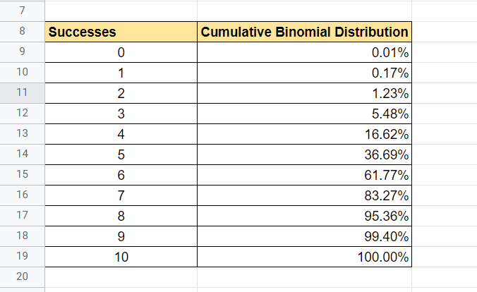
A cumulative binomial distribution is simply the sum of multiple binomial distributions. For example, if we would like to compute the probability for a coin to land on heads at least 9 out of 10 times, we have to consider scenarios where the coin lands nine times and when it lands all ten times.
To illustrate this concept further, let’s say you’re drafting basketball players based on how good they are at free throws. Let’s consider that a good basketball player has a 60% probability of a successful free throw. In this case, we can only give him 10 chances to make a free throw. We want to know the minimum number of shots the player needs to take to give us a 90% chance that he is a good player.
The CRITBINOM function can solve this quite easily. We just need to provide the number of independent trials (10 chances), the probability of success for each trial (60%), and the target probability (90%).
Let’s learn how to write the CRITBINOM function ourselves in Google Sheets.
The Anatomy of the CRITBINOM Function
The syntax of the CRITBINOM function is as follows:
=CRITBINOM(num_trials, prob_success, target_prob)
Let’s dissect this thing and understand what each of these terms means:
- = the equal sign is how we start any function in Google Sheets.
- CRITBINOM() is our
CRITBINOMfunction. It computes the smallest value for which the cumulative binomial distribution is greater than or equal to a specified criteria. - num_trials refers to the number of independent trials.
- prob_success refers to the probability of success in any given trial.
- target_prob refers to the desired threshold probability.
A Real Example of Using CRITBINOM Function
Let’s look at a specific example of the CRITBINOM function being used in a Google Sheets spreadsheet.
In the table below, we have a tabular version of the example laid out earlier. We have the number of free throws given to the player, the probability of successful free throws (for a “good” player), and the threshold of which to consider the player in the draft. Using CRITBINOM, we were able to come up with a result of 8 successful free throws to be part of the draft.

To get the value in cell B4, we just need to use the following formula:
=CRITBINOM(A2, B2, C2)
Using the BINOMDIST formula, we can verify the result of our CRITBINOM function. As seen in the table below, 8 successes out of 10 is the lowest number that is greater than or equal to the criterion of 90%.
You can make your own copy of the spreadsheet above using the link I have attached below.
If you’re ready to try out the CRITBINOM function in Google Sheets, let’s begin writing it ourselves!
Do you think you’re prepared to use the CRITBINOM function in Google Sheets? Head over to the next section to follow a step-by-step guide to using the function.
How to Use CRITBINOM Function in Google Sheets
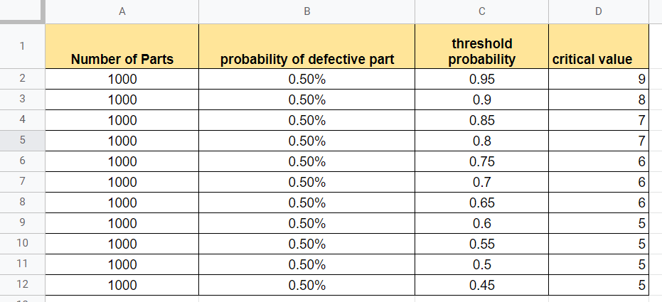
In this particular example, we’ll work with a scenario where you have an assembly line that generates parts. In this case, there is a 0.5% chance for any part to be considered defective. We want to know the critical values for various given thresholds. Each critical value will tell us how many parts per 1000 made do we accept until we have to shut down the assembly line.
- First, we must select the cell to write our
CRITBINOMfunction. In the table below, we can start with cell D2.

- Next, we just simply have to type the equal sign ‘=‘ to begin the function, followed by ‘CRITBINOM(‘.
- The next step is to type in our arguments. For the first row, we can find our arguments in order, giving us
CRITBINOM(A2, B2, C2). Afterward, simply hit Enter on your keyboard to let the function evaluate.

- Finally, we can drag down the formula in cell D2 to fill in the rest of the column.
That’s all you need to know on how to use the CRITBINOM function in Google Sheets. In conclusion, this article shows how easy it is to find critical values of a cumulative binomial distribution.
You can now use the CRITBINOM functions in Google Sheets together with the various other Google Sheets formulas available to create great worksheets that work for you.
Stay notified of new Google Sheets guides just like this by subscribing to our free newsletter!