How to Match Two Columns and Return a Third in Excel

This guide will discuss how to match two columns and return a third in Excel using three easy and simple methods. 

Since it has several built-in functions and features, Excel is a popular tool for dealing with data. And we can easily organize and manipulate data we input in Excel. Precisely, we can match two columns in Excel and return the third column containing data from any of the first two columns. 

Let’s take a sample scenario wherein we must match two columns and return a third in Excel.

Suppose you have created an employee directory containing the employee’s name and department. But, you want to be able to easily find an employee’s department without searching the entire directory. Essentially, you want to be able to input an employee and return their matching department. 

For instance, you are looking for a department of five employees, which you placed in another column. Then, you used the VLOOKUPfunction to match the two columns, which are the employee names from the directory and the employee names you are looking for. 

Afterward, the function will return the corresponding department of the employee you are looking for. 

Before we move on and discuss the three methods, let’s first learn how to write the functions we will be using in Excel.

The Anatomy of the VLOOKUP Function

The syntax or the way we write the VLOOKUP function is as follows:

=VLOOKUP(lookup_value, table_array, col_index_num, [range_lookup])

Let’s take apart this formula and understand what each term means:

• = the equal sign is how we start any function in Excel.
• VLOOKUP() is our VLOOKUP function. And this function is used to look for a value in the leftmost column of a table and return a value in the same row from a column we specify. 
• lookup_value is a required argument. So this refers to an existing value in the first column of the table. For instance, it can be a value, a cell reference, or a text string.
• table_array is another required argument. And this is a table of text, numbers, or logical values from which data is extracted. 
• col_index_num is also a required argument. So this refers to a column number from table_array from which the matching value should be returned. 
• range_lookup is an optional argument. And this is a logical value that indicates the kind of match to find. If TRUE or left blank, the function will return the closest match. If FALSE, it will find the exact match. 

The Anatomy of the INDEX Function

The syntax or the way we write the INDEX function is as follows:

=INDEX(array, row_num, [column_num])

Let’s take apart this formula and understand what each term means:

• = the equal sign is how we begin any function in Excel.
• INDEX() refers to our INDEX function. And this function is used to return a value or cell reference at the intersection of a specific row and column based on the given range.
• array is a required argument. So it refers to a range of cells or an array constant we select.
• row_num is also a required argument. And this will select the row in the array from which to return a value. When this is omitted, we need to input the column_num argument. 
• column_num is an optional argument. Similarly, this will select the column in the array from which to return a value. If omitted, the row_num argument is required. 

Great! Now we can explain how to match columns and return a third in Excel using three simple and easy methods.

How to Match Two Columns and Return a Third in Excel using the VLOOKUP Function

Firstly, we will utilize the VLOOKUP function to match two columns and return a third in Excel. Let’s say we have the same dataset from the sample scenario, which contains the employee name and department. 

So the VLOOKUP function will take a value from employee name-2 as the lookup value. Then, it will look for a match in the selected array, which is the employee name column. Lastly, it will return the corresponding department of the employee. 

To do this method, we can follow the steps below.

1. Firstly, we will create a new column beside Employee Name-2 to place the returned third column. Then, we will type in the formula “=VLOOKUP(E2,$B$2:$C$10,2,FALSE)”. Lastly, we will press the Enter key to return the value.

2. Secondly, we will drag down the Fill Handle tool to copy the formula and apply it to the rest of the cells.

3. And tada! We have successfully matched two columns and returned a third in Excel using the VLOOKUP function.

How to Match Two Columns and Return a Third in Excel using the INDEX and MATCH Functions

Secondly, we can use the INDEX and MATCH functions to perform the same task of matching two columns and returning a third in Excel. Additionally, we will be using the same dataset as the first method.

So the MATCH function returns the relative position of data in the selected array that matches a certain value in a specified order. In this case, the MATCH function will return the relative position of a value in employee name-2. 

Then, the INDEX function will take the output from the MATCH function to return the corresponding department. 

To use this method in your work, simply follow the steps discussed below.

1. Firstly, we will create a new column to input the results. So we will type in the formula “=INDEX($C$2:$C$10, MATCH(E2,$B$2:$B$10,0))”. Lastly, we will press the Enter key to return the result.

2. Next, we will drag the Fill Handle tool down to copy the formula to the rest of the column.

3. And tada! We have successfully used the INDEX-MATCH function to match two columns and return a third in Excel.

How to Match Two Columns and Return a Third in Excel using the IF, INDEX, and MATCH Functions

Lastly, we can combine the IF, INDEX, and MATCH functions to create a formula that will allow us to match two columns and return a third in Excel. In this case, we have altered the dataset a tiny bit. 

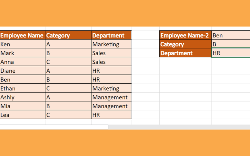
For example, we now have three columns in our employee directory: the employee name, category, and department. Furthermore, we will have two values to match: the employee name and the category. 

So the IF function will perform a logical test since we have an array condition. Then, the MATCH function will find the value in the selected array and return the relative position. Next, the INDEX function will return the value using the output from the MATCH function. 

To apply this method, we can use the steps mentioned below.

1. Firstly, we will input the necessary values to match. In this case, we have the employee’s name and category. Next, we will create an area to input the result.

So we will type in the formula “=INDEX(D13:D21,MATCH(G12,IF(C13:C21=G13,B13:B21,0)))”. Lastly, we will press the Enter key to return the result.

2. And tada! We have used the combination functions to perform the task.

You can make your own copy of the spreadsheet above using the link attached below. 

Amazing! We have discussed matching two columns and returning a third in Excel using three easy and simple ways. Now you can apply any of the methods to your work. 

Are you interested in learning more about what Excel can do? You can now use the VLOOKUP function and the various other Microsoft Excel formulas available to create great worksheets that work for you. Make sure to subscribe to our newsletter to be the first to know about the latest guides and tutorials from us.

Get emails from us about Google Sheets.

Our goal this year is to create lots of rich, bite-sized tutorials for Google Sheets users like you. If you liked this one, you'll love what we are working on! Readers receive ✨ early access ✨ to new content.

Subscribe