How to Remove Duplicates by Key Column in Google Sheets

This guide will explain how to remove duplicates by a key column in Google Sheets.

Google Sheets comes with multiple methods you can use to remove duplicates from a range of values. However, removing duplicate rows based on a specific key column can be challenging.

For example, you have a table of items where each one comes in multiple versions. In this case, you want to remove all duplicate items to achieve a final table that contains only one instance of each item.

This guide will look into the most effective methods in Google Sheets for removing duplicate entries by a given key column.

A Real Example of Removing Duplicates by Key Column in Google Sheets

Let’s explore a simple example where we must remove duplicates based on a table’s key column.

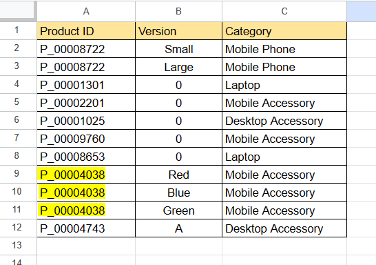
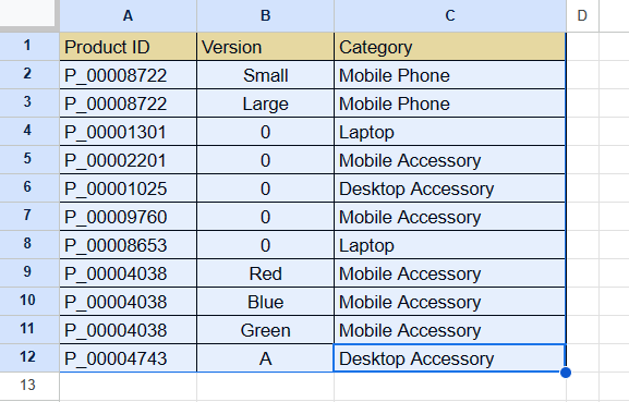
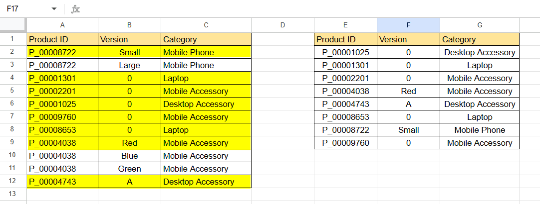
In the example above, we have a table that lists multiple products. Each product comes in one or more versions and is assigned a particular category. For example, the product with the product ID P_0004038 comes in three versions: Red, Blue, and Green.

We want to remove rows in our table to ensure each product ID  only appears once. We will also have to include the other two columns (B and C) from our range in our result. 

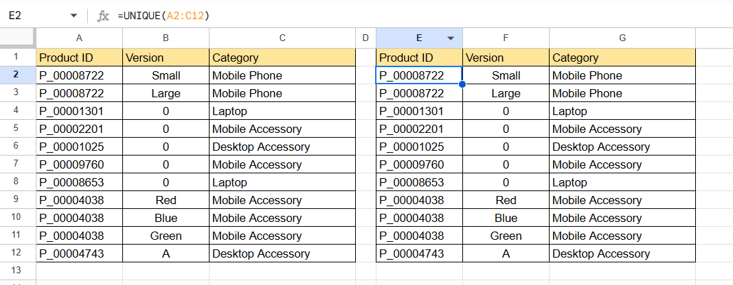
If we try to use the UNIQUE function on our range, the output will still return all our rows. The formula UNIQUE(A2:C12) considers the Version column, regardless if the value in the Product ID column is duplicated. 

A workaround to this issue is through the use of the Remove Duplicates feature. This feature allows us to limit which columns to analyze when detecting duplicates. In the image above, we will select our Product ID key column as the only column to consider when removing duplicates.

However, we have to note that the Remove Duplicates tool does not work dynamically. Users must use the tool manually every time new data is added. This method also permanently deletes duplicate values, which may not be compatible with some workflows.

A dynamic alternative you can use is the SORTN function. SORTN is used primarily for sorting datasets by the top or bottom N rows based on a certain column. However, adjusting the parameters of this function will allow you to remove duplicates from a range based on values from a single column.

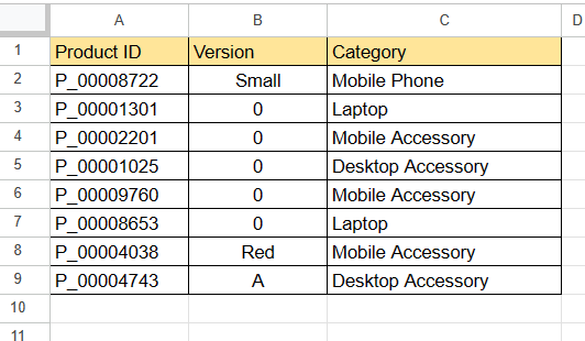
In the picture above, we created a new table of values where rows with duplicate Product ID values are removed. We can use the following formula to retrieve this result:

=SORTN(A2:C12,12,2,1,TRUE)

The SORTN function above analyzes the data in A2:C12 and returns the data sorted by the Product ID field. The third argument controls how the SORTN function handles duplicate rows. The method associated with ‘2’ retains the first instance and removes the succeeding duplicate rows.

While SORTN is effective in removing duplicate values, users should keep in mind that it modifies the order of the original dataset. Since the function must sort the data by the key column, this may result in a change to its initial order. 

You can make a copy of the spreadsheet above using the link attached below. 

Head over to the next section to follow our step-by-step tutorial on removing duplicates by a key column.

How to Remove Duplicates by Key Column in Google Sheets

Method 1: Using the Remove Duplicates Tool

1. First, select the range you want to remove duplicates from.
   
2. Next, head to the Data menu and click on Data cleanup then Remove Duplicates.
   
3. Check the option ‘Data has header row’ if applicable to your selection. Next, select the column to analyze to find duplicates. Click Remove duplicates to proceed.
   In this example, the Remove duplicates tool will only look for duplicates in Column A.
   
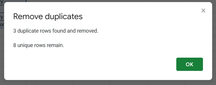
4. A pop-up will appear showing the number of duplicate rows found and removed. Click on OK to continue.
   
5. The selected range should now have no duplicate values in the selected key column.
   
   

Method 2: Using the SORTN Function

1. Select the cell where you want to output the filtered column.
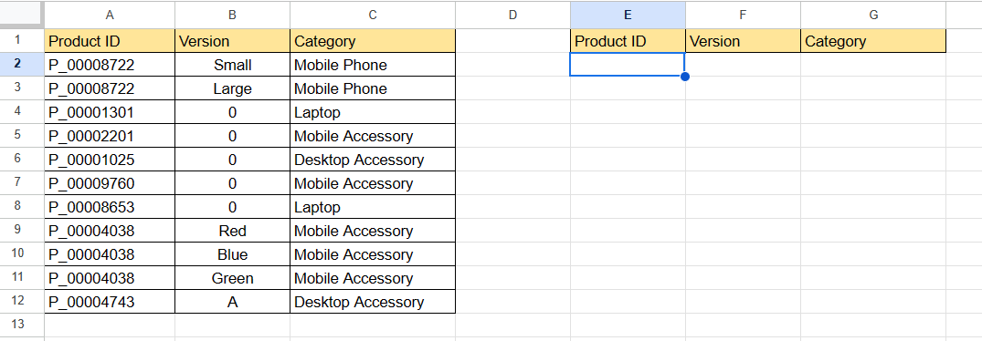   In the table above, we’ll select cell E2 so our formula result will populate the new table in columns E to G.
   
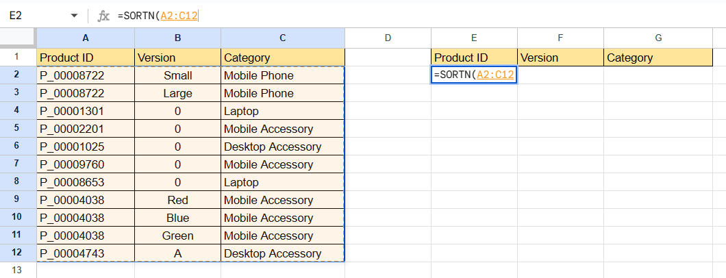
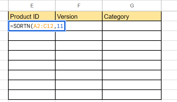
2. Type the string ‘=SORTN(‘ to start the function.
   
3. The first argument of SORTN determines what range the formula retrieves data from. In our example, we’ll select the range A2:C12.
   
4. SORTN’s second argument controls the number of items the formula will return. Since it is not yet clear how many unique rows remain after removing duplicates, placing the total number of rows in our range is the safest input.
   
5. By default, SORTN does not remove duplicate rows. Therefore, we must place a value of 2 in our third argument to force SORTN to remove duplicate rows from the result.
   
6. The fourth argument determines the index of the column in our selected range to use during the sorting. While the fifth argument indicates how to sort the chosen column. TRUE sorts in ascending order and FALSE sorts in descending order.
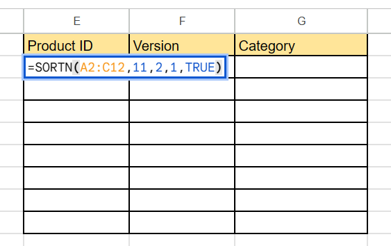   In our formula, we’ll type 1 in the fourth argument since our key column Product ID is the first column of our range. We’ll also set our formula to arrange the results in ascending order.
   
7. Hit the Enter key to evaluate the SORTN function. The formula should now return a copy of the table with all duplicates removed based on a given key column.
   

These are all the steps you need to follow to remove duplicates on a range based on a specified key column.

SORTN is just one of the many built-in functions available in Google Sheets. If you’re looking for another versatile way to filter and sort data, read our detailed guide on the FILTER function.

To learn more advanced spreadsheet techniques like this, try browsing our library of Google Sheets resources, tips, and tricks! 

Get emails from us about Google Sheets.

Our goal this year is to create lots of rich, bite-sized tutorials for Google Sheets users like you. If you liked this one, you'd love what we are working on! Readers receive early access to new content.

Subscribe